Dynamic hydrogen plant, amine unit, sulfur plant and crude unit

The refinery units of difflow_refinery are steady-state models. difflow_refinery.dynamic gives them the holdups that set how they move in time, and runs them on difflow’s dynamic framework (difflow.dynamic.DynamicFlowsheet). Example 66 did the hydrotreater and the reformer. This one does four more units, each built from its solved steady unit:

• DynamicHydrogenPlant (SMR): the reformer tubes as thermal cells (tube metal and catalyst heat capacity, the steady Xu-Froment tube equations across each cell), a furnace lag, the HT shift bed as equilibrium cells, and the PSA behind a cycle-averaged lag.

• DynamicAminePlant: the amine loop with its lean and rich solvent inventories; the steady unit’s lean-loading tear becomes their states.

• DynamicSRU: Claus converters and the TGTU hydrogenation reactor as equilibrium cells with catalyst heat capacity, reheater lags, the TGTU solvent inventory (the steady SRU’s recycle tear becomes a state), and air-demand control.

• DynamicCrudeUnit: the steady crude column between a furnace lag and the product inventories (reflux drum, side-stripper sumps, column bottom).

Each one starts at its steady unit’s state and rests there; every trajectory is differentiable. The holdup sizes, heat capacities and lags are illustrative design values: they set how fast things move, not where they settle. The gates (steady limit, balances along a trajectory, gradients against central differences, time scales) are in tests/reference/dynamic_utilities_checks.py and the docs’ “Dynamic operation” section.

import time
import warnings
import jax
jax.config.update("jax_enable_x64", True)
import jax.numpy as jnp
import numpy as np
import matplotlib.pyplot as plt

from difflow import make_stream
import difflow_refinery.hydrogen as h2
from difflow_refinery.dynamic import DynamicHydrogenPlant, DynamicAminePlant, DynamicSRU, SRUHoldupParams
from difflow_refinery.dynamic import DynamicCrudeUnit
H = 3600.0

1. The hydrogen plant

The docs’ SMR case: the IEAGHG 2017/02 natural gas, 240 tubes, S/C 2.75, reformer outlet 920 C, HT shift, a PSA at 90 % recovery. The tube is eight cells; each holds its share of the tube metal (HP alloy, 12.7 mm wall) and catalyst. The furnace lag is 5 minutes, the PSA lag 10 minutes.

y = {"methane": 0.89, "ethane": 0.07, "propane": 0.01, "n_butane": 0.0011,
     "carbon_dioxide": 0.02, "nitrogen": 0.0089, "hydrogen_sulfide": 5e-6}
natural_gas = make_stream({k: v * 1455.8 / 3.6 for k, v in y.items()}, 401.15, 3.71e6)
p = h2.SMRParams(n_tubes=240, psa=h2.PSA(recovery=0.90, purity=0.9999))
t0 = time.time()
plant = DynamicHydrogenPlant.from_steady(natural_gas, p)
print(f"built in {time.time() - t0:.0f} s: {plant.y0.size} states")
print(f"tube thermal time {plant.tau_tube / 60:.0f} min, shift bed {plant.tau_beds[0] / 60:.0f} min")
ob, ref = plant.observe(0.0, plant.y0), plant.steady_reference()
for k in ("H2", "T_reformer_out", "CH4_slip", "fuel"):
    print(f"{k:16s} dynamic at t=0 {float(ob[k]):.6g}   steady {float(ref[k]):.6g}")

built in 18 s: 29 states
tube thermal time 17 min, shift bed 10 min

H2               dynamic at t=0 1237.64   steady 1237.64
T_reformer_out   dynamic at t=0 1193.15   steady 1193.15
CH4_slip         dynamic at t=0 0.0357224   steady 0.0357224
fuel             dynamic at t=0 89.369   steady 89.369

Two upsets: the furnace fired 3 % harder at 10 minutes, then the natural gas cut 5 % at 1.5 hours with the firing held. The outlet temperature follows the firing through the furnace lag and the tube’s heat capacity; the product hydrogen follows the reformer and then the PSA.

Q0 = plant.base_signals["firing"]
a = plant.args(steps={"firing": [(600.0, 0.03 * Q0)], "feed_rate": [(1.5 * H, -0.05)]})
t0 = time.time()
sim = plant.simulate(3.5 * H, args=a, n_save=211)
tr = plant.trajectory(sim, a)
print(f"3.5 h in {time.time() - t0:.0f} s ({int(sim.info.n_steps)} steps)")
fig, ax = plt.subplots(1, 3, figsize=(13, 3.4))
t = np.asarray(tr["t"]) / H
ax[0].plot(t, np.asarray(tr["T_reformer_out"]) - 273.15); ax[0].set_ylabel("reformer outlet (C)")
ax[1].plot(t, np.asarray(tr["H2"]) * 2.016e-3 * 3.6); ax[1].set_ylabel("H2 product (t/h)")
ax[2].plot(t, 100 * np.asarray(tr["CH4_slip"])); ax[2].set_ylabel("CH4 slip (dry mol%)")
for x in ax: x.set_xlabel("time (h)")
plt.tight_layout()

3.5 h in 8 s (114 steps)

A gradient through the trajectory: how much more hydrogen an hour later per watt of extra firing at 5 minutes, by reverse mode through the diffrax solve and the tube cells’ own nested integrations.

def h2_at_1h(dQ):
    a = plant.args(steps={"firing": [(300.0, dQ)]})
    s = plant.simulate(H, args=a, n_save=2)
    return plant.observe(s.trajectory.t[-1], s.y_final, a)["H2"]

t0 = time.time()
g = jax.grad(h2_at_1h)(jnp.asarray(0.02 * Q0))
print(f"d(H2 at 1 h)/d(firing step) = {float(g) * 1e6:.4f} mol/s per MW ({time.time() - t0:.0f} s)")

d(H2 at 1 h)/d(firing step) = 7.6858 mol/s per MW (35 s)

2. The amine unit

The MDEA loop of the treating tests: one contactor on 980 mol/s of fuel gas with 2 % H2S and 2 % CO2, 120 mol/s of amine, a six-stage regenerator at 5 MW. The lean inventory holds 15 minutes of circulation, the rich one 10.

The sour gas rises 30 % at 5 minutes. The sweet gas’s H2S jumps at once (the contactor’s trays are quasi-steady), then keeps rising over the next hour as the more heavily loaded solvent comes back from the regenerator less well stripped.

from difflow_refinery.treating import TrayParams
from difflow_refinery.treating.unit import AmineUnitParams, Contactor
tray = TrayParams(area=200.0, k_G=1e-5, k_L=1e-4)        # ILLUSTRATIVE tray coefficients
loop = AmineUnitParams("MDEA", 0.45, (Contactor("fuel", 120.0, 8, tray),), Q_reboiler=5e6, n_regenerator=6)
gas = {"F_methane": 700.0, "F_ethane": 150.0, "F_hydrogen": 110.0, "F_hydrogen_sulfide": 20.0,
       "F_carbon_dioxide": 20.0, "F_water": 1.0, "T": 313.15, "P": 7e5}
t0 = time.time()
amine = DynamicAminePlant.from_steady(loop, {"fuel": gas})
print(f"built in {time.time() - t0:.0f} s (most of it the steady loop's solve and compile)")
a = amine.args(steps={"gas_rate": [(300.0, 0.3)], "Q_reboiler": [(2.0 * H, 1.0e6)]})
t0 = time.time()
sim = amine.simulate(4 * H, args=a, n_save=97)
ta = amine.trajectory(sim, a)
print(f"4 h in {time.time() - t0:.0f} s")
fig, ax = plt.subplots(1, 3, figsize=(13, 3.4))
t = np.asarray(ta["t"]) / H
ax[0].plot(t, ta["fuel.H2S_ppm"]); ax[0].set_ylabel("sweet gas H2S (ppm)")
ax[1].plot(t, ta["lean.alpha_H2S"], label="lean"); ax[1].set_ylabel("lean H2S loading")
ax[2].plot(t, ta["acid_gas.H2S"]); ax[2].set_ylabel("acid gas H2S (mol/s)")
for x in ax: x.set_xlabel("time (h)")
plt.tight_layout()

built in 95 s (most of it the steady loop's solve and compile)

4 h in 77 s

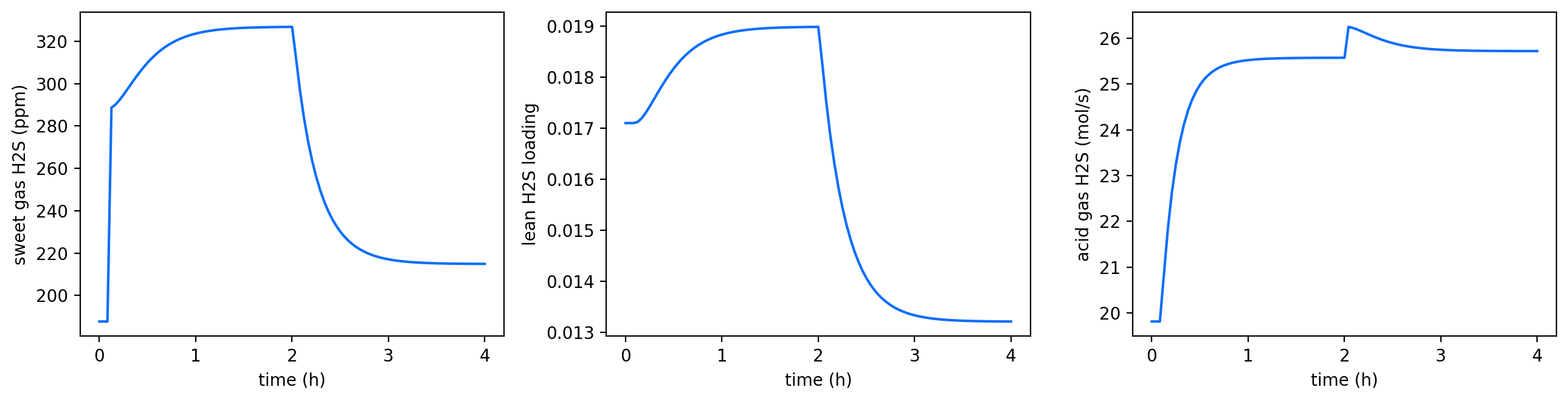
At 2 hours the reboiler duty is raised by 1 MW: the regenerator strips harder, and the lean loading – and with it the sweet gas – comes down over the lean inventory’s turnover.

3. The sulfur recovery unit

The SRU of the sulfur tests: 90 mol/s of H2S in the acid gas, two Claus beds, a SCOT tail-gas unit whose acid gas is recycled to the furnace. Each converter’s alumina is sized at a GHSV of 1000 1/h, so a bed holds about half an hour of thermal inventory.

The acid gas rises 10 % at 5 minutes. Run open loop (the air held at its design flow) the tail gas goes H2S-rich and the recovery falls; with the air-demand trim (an integral controller on the tail gas’s H2S - 2 SO2) the air follows the acid gas and the recovery comes back.

from difflow_refinery.sulfur import claus as cl, tgtu as tg
acid = make_stream({"hydrogen_sulfide": 90.0, "carbon_dioxide": 5.0, "water": 4.0, "methane": 1.0},
                   T=323.15, P=1.6e5)
beds = (cl.ConverterParams(523.15, hydrolysis=(0.9, 0.7)), cl.ConverterParams(483.15))
claus = cl.ClausParams(converters=beds, T_condensers=(443.15, 438.15, 413.15), T_air=473.15)
tgtu = tg.TGTUParams(tray=TrayParams(area=200.0, k_G=1e-5, k_L=1e-4), L=30.0, n_stages=12)
t0 = time.time()
sru = DynamicSRU.from_steady(acid, claus, tgtu)
sru_ctl = DynamicSRU.from_steady(acid, claus, tgtu, result=sru.steady, holdup=SRUHoldupParams(air_Ki=2e-3))
print(f"built in {time.time() - t0:.0f} s; bed thermal times "
      + ", ".join(f"{x / 60:.0f}" for x in sru.tau_beds) + " min (Claus 1, Claus 2, hydrogenation)")
a = sru.args(steps={"acid_rate": [(300.0, 0.1)]})
out = {}
for name, u in (("open loop", sru), ("air-demand control", sru_ctl)):
    t0 = time.time()
    s = u.simulate(3 * H, args=a, n_save=61)
    out[name] = u.trajectory(s, a)
    print(f"{name}: 3 h in {time.time() - t0:.0f} s")
fig, ax = plt.subplots(1, 3, figsize=(13, 3.4))
for name, tr_ in out.items():
    t = np.asarray(tr_["t"]) / H
    ax[0].plot(t, 100 * np.asarray(tr_["recovery"]), label=name)
    ax[1].plot(t, tr_["air"], label=name)
    ax[2].plot(t, np.asarray(tr_["bed1.T_out"]) - 273.15, label=name)
ax[0].set_ylabel("S recovery (%)"); ax[1].set_ylabel("air (mol/s)"); ax[2].set_ylabel("Claus bed 1 outlet (C)")
ax[0].legend()
for x in ax: x.set_xlabel("time (h)")
plt.tight_layout()

built in 199 s; bed thermal times 21, 25, 17 min (Claus 1, Claus 2, hydrogenation)

open loop: 3 h in 83 s

air-demand control: 3 h in 42 s

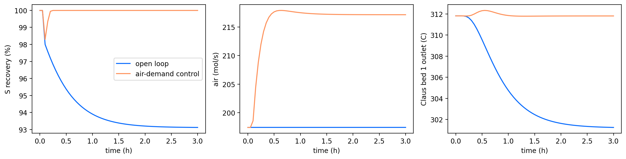
The bed outlet moves over tens of minutes: the thermal wave of the extra reaction heat crossing the alumina. The recycle from the TGTU follows its solvent inventory’s turnover.

4. The crude unit

The docs’ test crude at 95 000 bbl/d into the docs’ 30-stage column (three side strippers, two pumparounds). The column’s furnace spec, an overflash, is re-specified as the coil outlet temperature it solves to, held by a 10-minute furnace lag. Draws and pumparound duties follow the charge in proportion.

The coil outlet setpoint rises 5 K at 5 minutes, and the charge falls 5 % at 1.5 hours. The cut temperatures follow the furnace through their holdups; the cut rates follow the charge.

from difflow_refinery import Assay, ColumnThermo, characterize, column as cc
assay = Assay([0, 5, 10, 20, 30, 40, 50, 60, 70, 80, 90, 95, 100],
              [t + 273.15 for t in (-10, 60, 95, 150, 205, 260, 315, 370, 430, 500, 600, 680, 850)],
              sg=0.86, light_ends={"propane": 0.5, "n_butane": 1.0, "n_pentane": 1.5})
crude = characterize(assay)
thermo = ColumnThermo.from_characterization(crude)
kg_s = 95_000 * cc.BARREL / 86400.0 * float(crude.bulk_sg) * 999.016
feed = crude.stream(kg_s, T=273.15 + 240, P=6e5, basis="mass")
Vf = float(thermo.std_volume(jnp.stack([jnp.asarray(feed[f"F_{n}"]) for n in thermo.names])))
params = cc.CrudeColumnParams(
    n_stages=30, feed_stage=27, P_top=1.5e5, P_bottom=1.9e5, P_condenser=1.3e5,
    bottom_steam=150.0, steam_T=533.15,
    side_products=(cc.SideProduct("kero", 9, 4, steam=40.0), cc.SideProduct("diesel", 16, 4, steam=40.0),
                   cc.SideProduct("ago", 22, 3, steam=20.0)),
    pumparounds=(cc.Pumparound("pa1", 12, 10), cc.Pumparound("pa2", 19, 17)),
    specs=(cc.product_rate("naphtha", 0.20 * Vf), cc.product_rate("kero", 0.11 * Vf),
           cc.product_rate("diesel", 0.17 * Vf), cc.product_rate("ago", 0.05 * Vf),
           cc.pumparound_duty("pa1", 15e6), cc.pumparound_delta_t("pa1", 60.0),
           cc.pumparound_duty("pa2", 20e6), cc.pumparound_delta_t("pa2", 60.0), cc.overflash(0.05)),
    furnace=cc.Furnace(efficiency=0.85))
col = cc.CrudeColumn(params, thermo)
t0 = time.time()
cdu = DynamicCrudeUnit.from_steady(col, feed)
print(f"built in {time.time() - t0:.0f} s: coil outlet {float(cdu.base_signals['COT']) - 273.15:.1f} C")
a = cdu.args(steps={"COT": [(300.0, 5.0)], "feed_rate": [(1.5 * H, -0.05)]})
t0 = time.time()
sim = cdu.simulate(3 * H, args=a, n_save=61)
tc_ = cdu.trajectory(sim, a)
print(f"3 h in {time.time() - t0:.0f} s")
fig, ax = plt.subplots(1, 2, figsize=(10, 3.4))
t = np.asarray(tc_["t"]) / H
for n in ("kero", "diesel", "ago", "residue"):
    ax[0].plot(t, np.asarray(tc_[f"{n}.T"]) - np.asarray(tc_[f"{n}.T"])[0], label=n)
    ax[1].plot(t, np.asarray(tc_[f"{n}.volume"]) / np.asarray(tc_[f"{n}.volume"])[0], label=n)
ax[0].set_ylabel("product temperature change (K)"); ax[1].set_ylabel("product rate / initial")
ax[0].legend()
for x in ax: x.set_xlabel("time (h)")
plt.tight_layout()

built in 18 s: coil outlet 313.2 C

3 h in 133 s

What this does and does not show

• Every unit rests at its steady unit’s answer and returns to it after an upset (the gates quantify it); element or species balances close at every instant of every trajectory.

• The speeds are set by illustrative holdups and heat capacities. None of these transients has been compared with plant data or a published dynamic model.

• Not modelled: tray-by-tray column dynamics (the crude column, the amine contactor and regenerator are quasi-steady), pressure dynamics, a cycle-resolved PSA, wall heat in the sulfur plant’s furnace and condensers, and controllers other than the air-demand trim.