
Differentiable Programming Patterns#
This tutorial covers common patterns and techniques for differentiable programming, helping you choose the right approach for different problems.
Topics covered:
Unrolled vs implicit differentiation
Deep Equilibrium Models (DEQ)
Differentiating through argmin
Physics-informed constraints
Higher-order derivatives
Differentiable control flow
Soft operations and relaxations
Pattern selection guide
import jax
import jax.numpy as jnp
from jax import random, grad, jit, vmap, hessian, jacfwd, jacrev
from jax import lax
from jax import custom_vjp
import equinox as eqx
import optax
import optimistix as optx
import matplotlib.pyplot as plt
from functools import partial

jax.config.update("jax_enable_x64", True)

print(f"JAX version: {jax.__version__}")
WARNING:2026-01-10 20:59:22,940:jax._src.xla_bridge:852: An NVIDIA GPU may be present on this machine, but a CUDA-enabled jaxlib is not installed. Falling back to cpu.
JAX version: 0.8.2
1. Unrolled vs Implicit Differentiation#
When differentiating through iterative algorithms (optimization, fixed-point), you have two choices:
Unrolled differentiation:
Backprop through each iteration
Memory: O(iterations)
Exact for finite iterations
Implicit differentiation:
Use implicit function theorem at convergence
Memory: O(1)
Exact only at true fixed point
# Example: Fixed-point iteration x = tanh(Wx + b)

def fixed_point_unrolled(W, b, x0, n_iter=20):
    """
    Unrolled: backprop through all iterations.
    Memory grows with n_iter.
    """
    x = x0
    for _ in range(n_iter):
        x = jnp.tanh(W @ x + b)
    return x

@partial(custom_vjp, nondiff_argnums=(3, 4))
def fixed_point_implicit(W, b, x0, n_iter=20, tol=1e-6):
    """
    Implicit: only differentiate at convergence.
    Memory is O(1).
    """
    x = x0
    for _ in range(n_iter):
        x_new = jnp.tanh(W @ x + b)
        if jnp.max(jnp.abs(x_new - x)) < tol:
            break
        x = x_new
    return x

def fixed_point_implicit_fwd(W, b, x0, n_iter, tol):
    x_star = fixed_point_implicit(W, b, x0, n_iter, tol)
    return x_star, (W, b, x_star)

def fixed_point_implicit_bwd(n_iter, tol, res, g):
    """
    Implicit differentiation:
    x* = tanh(W @ x* + b)

    By implicit function theorem:
    dx*/dW = (I - J)^{-1} @ d(tanh)/dW
    where J = d(tanh(Wx+b))/dx = diag(1 - tanh²) @ W
    """
    W, b, x_star = res

    # Jacobian of tanh(Wx + b) w.r.t. x at x*
    tanh_val = jnp.tanh(W @ x_star + b)
    dtanh = 1 - tanh_val ** 2  # Derivative of tanh
    J = jnp.diag(dtanh) @ W  # d(tanh(Wx+b))/dx

    # Solve (I - J)^T @ v = g for v
    # This gives us the vector to backprop through
    v = jnp.linalg.solve((jnp.eye(len(x_star)) - J).T, g)

    # Gradients
    grad_W = jnp.outer(dtanh * v, x_star)
    grad_b = dtanh * v
    grad_x0 = jnp.zeros_like(x_star)  # Fixed point doesn't depend on x0

    return grad_W, grad_b, grad_x0

fixed_point_implicit.defvjp(fixed_point_implicit_fwd, fixed_point_implicit_bwd)

# Compare
key = random.PRNGKey(0)
n = 5
W = random.normal(key, (n, n)) * 0.5  # Small weights for convergence
b = random.normal(random.PRNGKey(1), (n,)) * 0.1
x0 = jnp.zeros(n)

x_unrolled = fixed_point_unrolled(W, b, x0)
x_implicit = fixed_point_implicit(W, b, x0)

print(f"Unrolled solution: {x_unrolled}")
print(f"Implicit solution: {x_implicit}")
print(f"Match: {jnp.allclose(x_unrolled, x_implicit, atol=1e-5)}")
Unrolled solution: [-0.30860964  0.08742608 -0.21691494  0.02575145 -0.062345  ]
Implicit solution: [-0.30860964  0.08742608 -0.21691494  0.02575145 -0.062345  ]
Match: True
# Compare gradients

def loss_unrolled(W, b, x0):
    x = fixed_point_unrolled(W, b, x0, n_iter=50)
    return jnp.sum(x ** 2)

def loss_implicit(W, b, x0):
    x = fixed_point_implicit(W, b, x0, n_iter=50)
    return jnp.sum(x ** 2)

grad_W_unrolled = grad(loss_unrolled)(W, b, x0)
grad_W_implicit = grad(loss_implicit)(W, b, x0)

print("Gradient comparison:")
print(f"  Unrolled grad norm: {jnp.linalg.norm(grad_W_unrolled):.6f}")
print(f"  Implicit grad norm: {jnp.linalg.norm(grad_W_implicit):.6f}")
print(f"  Difference: {jnp.linalg.norm(grad_W_unrolled - grad_W_implicit):.6f}")
Gradient comparison:
  Unrolled grad norm: 5.332211
  Implicit grad norm: 5.357392
  Difference: 0.030426
# When to use each?

print("""
UNROLLED DIFFERENTIATION:
✓ Few iterations (< 100)
✓ Need gradients at intermediate steps
✓ Non-convergent iterations matter
✗ High memory for many iterations
✗ Vanishing/exploding gradients possible

IMPLICIT DIFFERENTIATION:
✓ Many iterations needed
✓ Memory efficient (O(1))
✓ Stable gradients
✗ Requires true convergence
✗ Need to solve linear system
✗ More complex implementation

RECOMMENDATION:
- Use unrolled for training (few iterations, need intermediate grads)
- Use implicit for inference-time optimization
- Use optimistix for automatic implicit diff
""")
UNROLLED DIFFERENTIATION:
✓ Few iterations (< 100)
✓ Need gradients at intermediate steps
✓ Non-convergent iterations matter
✗ High memory for many iterations
✗ Vanishing/exploding gradients possible

IMPLICIT DIFFERENTIATION:
✓ Many iterations needed
✓ Memory efficient (O(1))
✓ Stable gradients
✗ Requires true convergence
✗ Need to solve linear system
✗ More complex implementation

RECOMMENDATION:
- Use unrolled for training (few iterations, need intermediate grads)
- Use implicit for inference-time optimization
- Use optimistix for automatic implicit diff
2. Deep Equilibrium Models (DEQ)#
DEQ models define the output as the fixed point of a neural network layer:
This is equivalent to an infinitely deep network with weight sharing!
# DEQ Layer using optimistix

class DEQLayer(eqx.Module):
    """
    Deep Equilibrium Layer.
    Output is fixed point: z* = f(z*, x)
    """
    linear1: eqx.nn.Linear
    linear2: eqx.nn.Linear
    input_proj: eqx.nn.Linear

    def __init__(self, input_dim, hidden_dim, *, key):
        keys = random.split(key, 3)
        self.input_proj = eqx.nn.Linear(input_dim, hidden_dim, key=keys[0])
        self.linear1 = eqx.nn.Linear(hidden_dim, hidden_dim, key=keys[1])
        self.linear2 = eqx.nn.Linear(hidden_dim, hidden_dim, key=keys[2])

    def f(self, z, x_proj):
        """One iteration: z_{k+1} = f(z_k, x)"""
        h = jax.nn.relu(self.linear1(z) + x_proj)
        return 0.5 * jnp.tanh(self.linear2(h))  # Contraction factor

    def __call__(self, x):
        # Project input
        x_proj = self.input_proj(x)

        # Find fixed point using optimistix
        def residual(z, args):
            return self.f(z, x_proj) - z

        z0 = jnp.zeros(x_proj.shape)
        solver = optx.Newton(rtol=1e-5, atol=1e-5)
        sol = optx.root_find(residual, solver, z0, max_steps=50, throw=False)

        return sol.value

# Test DEQ layer
key = random.PRNGKey(42)
deq = DEQLayer(input_dim=4, hidden_dim=8, key=key)

x = random.normal(key, (4,))
z_star = deq(x)

print(f"Input shape: {x.shape}")
print(f"Fixed point shape: {z_star.shape}")
print(f"Fixed point: {z_star}")

# Verify it's a fixed point
x_proj = deq.input_proj(x)
z_next = deq.f(z_star, x_proj)
print(f"\n|f(z*) - z*| = {jnp.max(jnp.abs(z_next - z_star)):.2e}")
Input shape: (4,)
Fixed point shape: (8,)
Fixed point: [ 0.03467625 -0.08210178  0.07491626 -0.12856947  0.16261056  0.19624736
 -0.08700007 -0.27254499]
|f(z*) - z*| = 1.67e-16
# Train DEQ model

class DEQClassifier(eqx.Module):
    deq: DEQLayer
    output: eqx.nn.Linear

    def __init__(self, input_dim, hidden_dim, output_dim, *, key):
        keys = random.split(key, 2)
        self.deq = DEQLayer(input_dim, hidden_dim, key=keys[0])
        self.output = eqx.nn.Linear(hidden_dim, output_dim, key=keys[1])

    def __call__(self, x):
        z = self.deq(x)
        return self.output(z)

# Create model and test gradient
model = DEQClassifier(input_dim=4, hidden_dim=8, output_dim=2, key=random.PRNGKey(0))

def loss_fn(model, x, y):
    logits = model(x)
    return jnp.sum((logits - y) ** 2)

x = random.normal(random.PRNGKey(1), (4,))
y = jnp.array([1.0, 0.0])

# Gradient flows through fixed point!
loss, grads = eqx.filter_value_and_grad(loss_fn)(model, x, y)

print(f"Loss: {loss:.4f}")
print(f"Gradient exists for DEQ layer: {grads.deq.linear1.weight is not None}")
print(f"DEQ linear1 grad norm: {jnp.linalg.norm(grads.deq.linear1.weight):.4f}")
Loss: 0.6543
Gradient exists for DEQ layer: True
DEQ linear1 grad norm: 0.0153
3. Differentiating Through Argmin#
Many problems involve optimization as a layer:
We want \(\frac{dy^*}{d\theta}\). By implicit differentiation at the optimum:
# Example: Quadratic optimization layer
# y* = argmin_y (1/2 y^T Q y - c^T y)
# Solution: y* = Q^{-1} c

def quadratic_layer_explicit(Q, c):
    """Direct solution (when available)."""
    return jnp.linalg.solve(Q, c)

def quadratic_layer_optx(Q, c):
    """Using optimistix minimization."""
    def objective(y, args):
        Q, c = args
        return 0.5 * y @ Q @ y - c @ y

    y0 = jnp.zeros_like(c)
    solver = optx.BFGS(rtol=1e-6, atol=1e-6)
    sol = optx.minimise(objective, solver, y0, args=(Q, c), max_steps=100)
    return sol.value

# Test
n = 3
key = random.PRNGKey(0)
A = random.normal(key, (n, n))
Q = A @ A.T + jnp.eye(n)  # Positive definite
c = random.normal(random.PRNGKey(1), (n,))

y_explicit = quadratic_layer_explicit(Q, c)
y_optx = quadratic_layer_optx(Q, c)

print(f"Explicit: {y_explicit}")
print(f"Optimistix: {y_optx}")
print(f"Match: {jnp.allclose(y_explicit, y_optx, atol=1e-4)}")
Explicit: [-0.28116662 -0.29375909  0.05391175]
Optimistix: [-0.28116662 -0.29375909  0.05391175]
Match: True
# Gradient through argmin

def loss_with_argmin(Q, c, target):
    y_star = quadratic_layer_optx(Q, c)
    return jnp.sum((y_star - target) ** 2)

target = jnp.ones(n)

# Gradient w.r.t. c (easier case)
grad_c = grad(loss_with_argmin, argnums=1)(Q, c, target)
print(f"Gradient w.r.t. c: {grad_c}")

# Verify: dy*/dc = Q^{-1}, so dL/dc = 2(y* - target)^T Q^{-1}
y_star = quadratic_layer_optx(Q, c)
expected_grad_c = 2 * jnp.linalg.solve(Q.T, y_star - target)
print(f"Expected gradient: {expected_grad_c}")
print(f"Match: {jnp.allclose(grad_c, expected_grad_c, atol=1e-3)}")
Gradient w.r.t. c: [-0.99139051 -2.7250085 -0.64922416]
Expected gradient: [-0.99139051 -2.7250085  -0.64922416]
Match: True
# Constrained optimization layer
# y* = argmin_y ||y - c||^2 subject to Ay = b

def projection_layer(c, A, b):
    """
    Project c onto affine subspace {y : Ay = b}.
    Uses optimistix least squares.
    """
    def residual(y, args):
        c, A, b = args
        # Penalized objective: ||y - c||^2 + large * ||Ay - b||^2
        return jnp.concatenate([y - c, 100 * (A @ y - b)])

    y0 = c
    solver = optx.LevenbergMarquardt(rtol=1e-6, atol=1e-6)
    sol = optx.least_squares(residual, solver, y0, args=(c, A, b), max_steps=100)
    return sol.value

# Example: project onto plane x + y + z = 1
A = jnp.array([[1.0, 1.0, 1.0]])
b = jnp.array([1.0])
c = jnp.array([2.0, 0.0, 0.0])  # Point to project

y_proj = projection_layer(c, A, b)

print(f"Original point: {c}")
print(f"Projected point: {y_proj}")
print(f"Constraint Ay: {A @ y_proj} (should be {b})")

# Gradient flows through projection!
def proj_loss(c, A, b):
    y = projection_layer(c, A, b)
    return jnp.sum(y ** 2)

grad_c = grad(proj_loss)(c, A, b)
print(f"\nGradient w.r.t. c: {grad_c}")
Original point: [2. 0. 0.]
Projected point: [ 1.66667778 -0.33332222 -0.33332222]
Constraint Ay: [1.00003333] (should be [1.])
Gradient w.r.t. c: [ 2.66668889 -1.33331111 -1.33331111]
4. Physics-Informed Constraints#
Embed physical constraints directly into differentiable models.
# Pattern 1: Soft constraints via penalty

def physics_loss_soft(params, x, y_data):
    """
    Soft constraint: add penalty term.
    Example: Mass conservation sum(y) = sum(x)
    """
    y_pred = model_fn(params, x)  # Some model

    # Data loss
    data_loss = jnp.mean((y_pred - y_data) ** 2)

    # Physics constraint penalty
    mass_violation = jnp.sum(y_pred) - jnp.sum(x)
    physics_loss = 1000 * mass_violation ** 2

    return data_loss + physics_loss

print("Soft constraints: Add penalty term")
print("+ Simple to implement")
print("+ Works with any constraint")
print("- Constraint only approximately satisfied")
print("- Need to tune penalty weight")
Soft constraints: Add penalty term
+ Simple to implement
+ Works with any constraint
- Constraint only approximately satisfied
- Need to tune penalty weight
# Pattern 2: Hard constraints via reparameterization

def enforce_mass_conservation(raw_output, total_mass):
    """
    Hard constraint: normalize to conserve mass.
    This is differentiable!
    """
    # Ensure non-negative
    positive_output = jax.nn.softplus(raw_output)
    # Normalize to sum to total_mass
    return positive_output / jnp.sum(positive_output) * total_mass

def enforce_positivity(x):
    """Ensure x > 0 via softplus."""
    return jax.nn.softplus(x)

def enforce_bounds(x, low, high):
    """Ensure low < x < high via sigmoid."""
    return low + (high - low) * jax.nn.sigmoid(x)

def enforce_simplex(logits):
    """Ensure x >= 0 and sum(x) = 1 via softmax."""
    return jax.nn.softmax(logits)

# Example
raw = jnp.array([1.0, -0.5, 2.0, 0.3])
total_mass = 10.0

conserved = enforce_mass_conservation(raw, total_mass)
print(f"Raw output: {raw}")
print(f"Conserved output: {conserved}")
print(f"Sum: {jnp.sum(conserved):.6f} (target: {total_mass})")

# Gradient flows through constraint!
grad_raw = grad(lambda r: jnp.sum(enforce_mass_conservation(r, total_mass) ** 2))(raw)
print(f"\nGradient w.r.t. raw: {grad_raw}")
Raw output: [ 1.  -0.5  2.   0.3]
Conserved output: [2.75396479 0.9941593  4.46025716 1.79161875]
Sum: 10.000000 (target: 10.0)
Gradient w.r.t. raw: [-1.26839861 -3.44158073 4.77508003 -3.31520906]
# Pattern 3: Conservation via architecture

class ConservativeNetwork(eqx.Module):
    """
    Network that inherently conserves mass.
    Outputs redistribution matrix, not absolute values.
    """
    layers: list

    def __init__(self, n_species, hidden_dim, *, key):
        keys = random.split(key, 3)
        self.layers = [
            eqx.nn.Linear(n_species, hidden_dim, key=keys[0]),
            eqx.nn.Linear(hidden_dim, hidden_dim, key=keys[1]),
            eqx.nn.Linear(hidden_dim, n_species * n_species, key=keys[2]),
        ]

    def __call__(self, x):
        """x: input composition, returns output composition."""
        n = len(x)

        # Compute redistribution logits
        h = x
        for layer in self.layers[:-1]:
            h = jax.nn.relu(layer(h))
        logits = self.layers[-1](h).reshape(n, n)

        # Softmax over columns: each column sums to 1
        # R[i,j] = fraction of species j that becomes species i
        R = jax.nn.softmax(logits, axis=0)

        # Apply redistribution: y = R @ x
        # This conserves mass: sum(y) = sum(R @ x) = sum(x) since columns sum to 1
        return R @ x

# Test
net = ConservativeNetwork(n_species=4, hidden_dim=16, key=random.PRNGKey(0))
x = jnp.array([10.0, 5.0, 3.0, 2.0])  # Total = 20

y = net(x)
print(f"Input: {x}, sum = {jnp.sum(x)}")
print(f"Output: {y}, sum = {jnp.sum(y):.6f}")
print(f"Mass conserved: {jnp.allclose(jnp.sum(x), jnp.sum(y))}")
Input: [10.  5.  3.  2.], sum = 20.0
Output: [5.46178306 3.54354348 5.44448837 5.55018509], sum = 20.000000
Mass conserved: True
5. Higher-Order Derivatives#
JAX supports arbitrary-order derivatives through nested transformations.
# Hessian computation

def f(x):
    """Rosenbrock function."""
    return (1 - x[0])**2 + 100 * (x[1] - x[0]**2)**2

x = jnp.array([0.5, 0.5])

# First derivative (gradient)
gradient = grad(f)(x)

# Second derivative (Hessian) - multiple ways
hess1 = hessian(f)(x)  # Direct
hess2 = jacfwd(jacrev(f))(x)  # Forward-over-reverse
hess3 = jacrev(jacfwd(f))(x)  # Reverse-over-forward

print(f"Gradient: {gradient}")
print(f"\nHessian (direct):")
print(hess1)
print(f"\nAll methods match: {jnp.allclose(hess1, hess2) and jnp.allclose(hess1, hess3)}")
Gradient: [-51.  50.]

Hessian (direct):
[[ 102. -200.]
 [-200.  200.]]

All methods match: True
# Hessian-vector product (efficient for large problems)

def hvp(f, x, v):
    """Compute Hessian-vector product: H @ v."""
    return grad(lambda x: jnp.dot(grad(f)(x), v))(x)

v = jnp.array([1.0, 0.0])
hvp_result = hvp(f, x, v)

# Verify against full Hessian
expected = hess1 @ v

print(f"HVP result: {hvp_result}")
print(f"H @ v:      {expected}")
print(f"Match: {jnp.allclose(hvp_result, expected)}")

print("\nHVP is O(n) while full Hessian is O(n²)!")
HVP result: [ 102. -200.]
H @ v:      [ 102. -200.]
Match: True

HVP is O(n) while full Hessian is O(n²)!
# Newton's method using Hessian

def newton_step(f, x):
    """One step of Newton's method."""
    g = grad(f)(x)
    H = hessian(f)(x)
    return x - jnp.linalg.solve(H, g)

# Optimize Rosenbrock
x = jnp.array([0.0, 0.0])
print("Newton's method on Rosenbrock:")
for i in range(10):
    x = newton_step(f, x)
    print(f"  Step {i+1}: x = [{x[0]:.6f}, {x[1]:.6f}], f(x) = {f(x):.2e}")

print(f"\nOptimum: [1, 1], found: [{x[0]:.6f}, {x[1]:.6f}]")
Newton's method on Rosenbrock:
  Step 1: x = [1.000000, 0.000000], f(x) = 1.00e+02
  Step 2: x = [1.000000, 1.000000], f(x) = 0.00e+00
  Step 3: x = [1.000000, 1.000000], f(x) = 0.00e+00
  Step 4: x = [1.000000, 1.000000], f(x) = 0.00e+00
  Step 5: x = [1.000000, 1.000000], f(x) = 0.00e+00
  Step 6: x = [1.000000, 1.000000], f(x) = 0.00e+00
  Step 7: x = [1.000000, 1.000000], f(x) = 0.00e+00
  Step 8: x = [1.000000, 1.000000], f(x) = 0.00e+00
  Step 9: x = [1.000000, 1.000000], f(x) = 0.00e+00
  Step 10: x = [1.000000, 1.000000], f(x) = 0.00e+00

Optimum: [1, 1], found: [1.000000, 1.000000]
# Third and higher derivatives

def g(x):
    return jnp.sin(x)

x = 0.5

# Derivatives of sin(x)
d1 = grad(g)(x)                    # cos(x)
d2 = grad(grad(g))(x)              # -sin(x)
d3 = grad(grad(grad(g)))(x)        # -cos(x)
d4 = grad(grad(grad(grad(g))))(x)  # sin(x)

print(f"f(x) = sin(x) at x = {x}")
print(f"f(x)   = {g(x):.6f} (sin)")
print(f"f'(x)  = {d1:.6f} (cos)")
print(f"f''(x) = {d2:.6f} (-sin)")
print(f"f'''(x)= {d3:.6f} (-cos)")
print(f"f''''(x)={d4:.6f} (sin)")
f(x) = sin(x) at x = 0.5
f(x)   = 0.479426 (sin)
f'(x)  = 0.877583 (cos)
f''(x) = -0.479426 (-sin)
f'''(x)= -0.877583 (-cos)
f''''(x)=0.479426 (sin)
6. Differentiable Control Flow#
JAX provides differentiable versions of control flow: lax.cond, lax.switch, lax.while_loop, lax.fori_loop.
# lax.cond - differentiable if-else

def cond_example(x, threshold):
    """
    Different computation based on condition.
    Gradient flows through the taken branch.
    """
    return lax.cond(
        x > threshold,
        lambda x: x ** 2,      # True branch
        lambda x: 2 * x,       # False branch
        x
    )

# Test
print("lax.cond example: f(x) = x² if x > 0.5 else 2x")
for x in [0.3, 0.7]:
    x = jnp.array(x)
    y = cond_example(x, 0.5)
    dy = grad(cond_example)(x, 0.5)
    print(f"  x = {x}: f(x) = {y:.3f}, f'(x) = {dy:.3f}")
lax.cond example: f(x) = x² if x > 0.5 else 2x
  x = 0.3: f(x) = 0.600, f'(x) = 2.000
  x = 0.7: f(x) = 0.490, f'(x) = 1.400
# lax.switch - differentiable multi-way branch

def switch_example(x, mode):
    """
    Select computation based on integer mode.
    """
    branches = [
        lambda x: x,           # Mode 0: identity
        lambda x: x ** 2,      # Mode 1: square
        lambda x: jnp.sin(x),  # Mode 2: sin
        lambda x: jnp.exp(x),  # Mode 3: exp
    ]
    return lax.switch(mode, branches, x)

x = jnp.array(0.5)
print("lax.switch example:")
for mode in range(4):
    y = switch_example(x, mode)
    dy = grad(switch_example)(x, mode)
    names = ['identity', 'square', 'sin', 'exp']
    print(f"  Mode {mode} ({names[mode]}): f({x}) = {y:.4f}, f'({x}) = {dy:.4f}")
lax.switch example:
  Mode 0 (identity): f(0.5) = 0.5000, f'(0.5) = 1.0000
  Mode 1 (square): f(0.5) = 0.2500, f'(0.5) = 1.0000
  Mode 2 (sin): f(0.5) = 0.4794, f'(0.5) = 0.8776
  Mode 3 (exp): f(0.5) = 1.6487, f'(0.5) = 1.6487
# Pattern: Soft switching (always differentiable)

def soft_switch(x, weights):
    """
    Weighted combination of branches.
    Differentiable w.r.t. both x and weights.
    """
    branches = jnp.array([
        x,
        x ** 2,
        jnp.sin(x),
        jnp.exp(x)
    ])
    # Soft weights via softmax
    soft_weights = jax.nn.softmax(weights)
    return jnp.sum(soft_weights * branches)

x = jnp.array(0.5)
weights = jnp.array([0.0, 1.0, 0.0, 0.0])  # Prefer square

y = soft_switch(x, weights)
grad_x = grad(soft_switch)(x, weights)
grad_w = grad(soft_switch, argnums=1)(x, weights)

print("Soft switch (all branches contribute):")
print(f"  Output: {y:.4f}")
print(f"  d/dx: {grad_x:.4f}")
print(f"  d/dweights: {grad_w}")
Soft switch (all branches contribute):
  Output: 0.5784
  d/dx: 1.0920
  d/dweights: [-0.01371846 -0.15613235 -0.01731647  0.18716728]
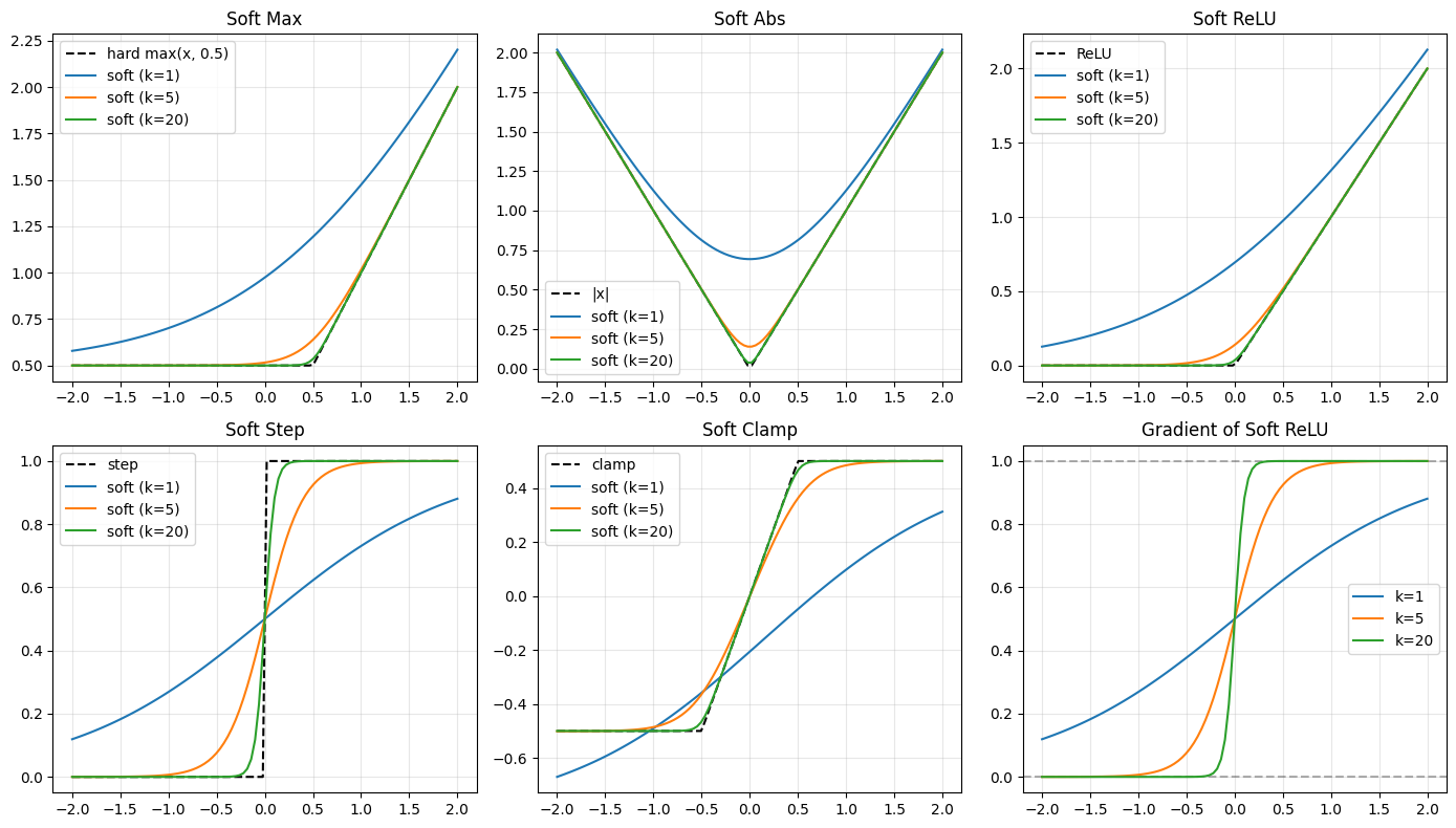
7. Soft Operations and Relaxations#
Replace non-differentiable operations with smooth approximations.
# Soft operations collection

def soft_max(a, b, sharpness=10.0):
    """Smooth approximation to max(a, b)."""
    return jax.nn.logsumexp(jnp.array([a, b]) * sharpness) / sharpness

def soft_min(a, b, sharpness=10.0):
    """Smooth approximation to min(a, b)."""
    return -soft_max(-a, -b, sharpness)

def soft_abs(x, sharpness=10.0):
    """Smooth approximation to |x|."""
    return soft_max(x, -x, sharpness)

def soft_relu(x, sharpness=10.0):
    """Smooth approximation to max(0, x)."""
    return soft_max(x, 0.0, sharpness)

def soft_step(x, sharpness=10.0):
    """Smooth approximation to step function (0 if x<0, 1 if x>0)."""
    return jax.nn.sigmoid(sharpness * x)

def soft_clamp(x, low, high, sharpness=10.0):
    """Smooth approximation to clamp(x, low, high)."""
    return soft_min(soft_max(x, low, sharpness), high, sharpness)

# Visualize
x = jnp.linspace(-2, 2, 100)

fig, axes = plt.subplots(2, 3, figsize=(14, 8))

# Max
axes[0, 0].plot(x, jnp.maximum(x, 0.5), 'k--', label='hard max(x, 0.5)')
for s in [1, 5, 20]:
    axes[0, 0].plot(x, vmap(lambda xi: soft_max(xi, 0.5, s))(x), label=f'soft (k={s})')
axes[0, 0].legend()
axes[0, 0].set_title('Soft Max')
axes[0, 0].grid(True, alpha=0.3)

# Abs
axes[0, 1].plot(x, jnp.abs(x), 'k--', label='|x|')
for s in [1, 5, 20]:
    axes[0, 1].plot(x, vmap(lambda xi: soft_abs(xi, s))(x), label=f'soft (k={s})')
axes[0, 1].legend()
axes[0, 1].set_title('Soft Abs')
axes[0, 1].grid(True, alpha=0.3)

# ReLU
axes[0, 2].plot(x, jnp.maximum(x, 0), 'k--', label='ReLU')
for s in [1, 5, 20]:
    axes[0, 2].plot(x, vmap(lambda xi: soft_relu(xi, s))(x), label=f'soft (k={s})')
axes[0, 2].legend()
axes[0, 2].set_title('Soft ReLU')
axes[0, 2].grid(True, alpha=0.3)

# Step
axes[1, 0].plot(x, (x > 0).astype(float), 'k--', label='step')
for s in [1, 5, 20]:
    axes[1, 0].plot(x, vmap(lambda xi: soft_step(xi, s))(x), label=f'soft (k={s})')
axes[1, 0].legend()
axes[1, 0].set_title('Soft Step')
axes[1, 0].grid(True, alpha=0.3)

# Clamp
axes[1, 1].plot(x, jnp.clip(x, -0.5, 0.5), 'k--', label='clamp')
for s in [1, 5, 20]:
    axes[1, 1].plot(x, vmap(lambda xi: soft_clamp(xi, -0.5, 0.5, s))(x), label=f'soft (k={s})')
axes[1, 1].legend()
axes[1, 1].set_title('Soft Clamp')
axes[1, 1].grid(True, alpha=0.3)

# Gradients of soft ReLU
axes[1, 2].axhline(0, color='k', linestyle='--', alpha=0.3)
axes[1, 2].axhline(1, color='k', linestyle='--', alpha=0.3)
for s in [1, 5, 20]:
    grads = vmap(grad(lambda xi: soft_relu(xi, s)))(x)
    axes[1, 2].plot(x, grads, label=f'k={s}')
axes[1, 2].legend()
axes[1, 2].set_title('Gradient of Soft ReLU')
axes[1, 2].grid(True, alpha=0.3)

plt.tight_layout()
plt.show()
8. Pattern Selection Guide#
Quick reference for choosing the right pattern.
print("""
╔══════════════════════════════════════════════════════════════════════════════╗
║                    DIFFERENTIABLE PROGRAMMING PATTERN GUIDE                   ║
╠══════════════════════════════════════════════════════════════════════════════╣
║                                                                              ║
║  ITERATIVE ALGORITHMS                                                        ║
║  ───────────────────                                                         ║
║  • Few iterations (<100): Unrolled differentiation                          ║
║  • Many iterations: Implicit differentiation                                 ║
║  • Fixed-point problems: optimistix.fixed_point                             ║
║  • Root finding: optimistix.root_find                                       ║
║                                                                              ║
║  OPTIMIZATION LAYERS                                                         ║
║  ───────────────────                                                         ║
║  • Unconstrained: optimistix.minimise                                       ║
║  • Least squares: optimistix.least_squares                                  ║
║  • Quadratic: Closed form + implicit diff                                   ║
║  • General constrained: Penalty method or projection                        ║
║                                                                              ║
║  PHYSICS CONSTRAINTS                                                         ║
║  ──────────────────                                                          ║
║  • Soft: Penalty in loss function                                           ║
║  • Hard via output: Reparameterization (softmax, sigmoid)                   ║
║  • Hard via architecture: Design conservation into network                  ║
║                                                                              ║
║  DISCRETE OPERATIONS                                                         ║
║  ───────────────────                                                         ║
║  • Categorical sampling: Gumbel-softmax                                     ║
║  • Hard selection: Straight-through estimator                               ║
║  • Comparisons: Soft approximations (sigmoid)                               ║
║  • Sorting/ranking: Soft sort or relaxed permutation                        ║
║                                                                              ║
║  CONTROL FLOW                                                                ║
║  ────────────                                                                ║
║  • Conditional: lax.cond (gradient through taken branch)                    ║
║  • Multi-branch: lax.switch                                                 ║
║  • Need all branch grads: Soft switch with softmax weights                  ║
║                                                                              ║
║  HIGHER-ORDER DERIVATIVES                                                    ║
║  ────────────────────────                                                    ║
║  • Full Hessian: jax.hessian(f)                                             ║
║  • Hessian-vector product: grad(lambda x: dot(grad(f)(x), v))              ║
║  • Mixed partials: jacfwd(jacrev(f))                                       ║
║                                                                              ║
║  MEMORY EFFICIENCY                                                           ║
║  ─────────────────                                                           ║
║  • Deep networks: jax.checkpoint / jax.remat                                ║
║  • Long sequences: Hierarchical checkpointing                               ║
║  • ODE gradients: diffrax.RecursiveCheckpointAdjoint                        ║
║                                                                              ║
╚══════════════════════════════════════════════════════════════════════════════╝
""")
╔══════════════════════════════════════════════════════════════════════════════╗
║                    DIFFERENTIABLE PROGRAMMING PATTERN GUIDE                   ║
╠══════════════════════════════════════════════════════════════════════════════╣
║                                                                              ║
║  ITERATIVE ALGORITHMS                                                        ║
║  ───────────────────                                                         ║
║  • Few iterations (<100): Unrolled differentiation                          ║
║  • Many iterations: Implicit differentiation                                 ║
║  • Fixed-point problems: optimistix.fixed_point                             ║
║  • Root finding: optimistix.root_find                                       ║
║                                                                              ║
║  OPTIMIZATION LAYERS                                                         ║
║  ───────────────────                                                         ║
║  • Unconstrained: optimistix.minimise                                       ║
║  • Least squares: optimistix.least_squares                                  ║
║  • Quadratic: Closed form + implicit diff                                   ║
║  • General constrained: Penalty method or projection                        ║
║                                                                              ║
║  PHYSICS CONSTRAINTS                                                         ║
║  ──────────────────                                                          ║
║  • Soft: Penalty in loss function                                           ║
║  • Hard via output: Reparameterization (softmax, sigmoid)                   ║
║  • Hard via architecture: Design conservation into network                  ║
║                                                                              ║
║  DISCRETE OPERATIONS                                                         ║
║  ───────────────────                                                         ║
║  • Categorical sampling: Gumbel-softmax                                     ║
║  • Hard selection: Straight-through estimator                               ║
║  • Comparisons: Soft approximations (sigmoid)                               ║
║  • Sorting/ranking: Soft sort or relaxed permutation                        ║
║                                                                              ║
║  CONTROL FLOW                                                                ║
║  ────────────                                                                ║
║  • Conditional: lax.cond (gradient through taken branch)                    ║
║  • Multi-branch: lax.switch                                                 ║
║  • Need all branch grads: Soft switch with softmax weights                  ║
║                                                                              ║
║  HIGHER-ORDER DERIVATIVES                                                    ║
║  ────────────────────────                                                    ║
║  • Full Hessian: jax.hessian(f)                                             ║
║  • Hessian-vector product: grad(lambda x: dot(grad(f)(x), v))              ║
║  • Mixed partials: jacfwd(jacrev(f))                                       ║
║                                                                              ║
║  MEMORY EFFICIENCY                                                           ║
║  ─────────────────                                                           ║
║  • Deep networks: jax.checkpoint / jax.remat                                ║
║  • Long sequences: Hierarchical checkpointing                               ║
║  • ODE gradients: diffrax.RecursiveCheckpointAdjoint                        ║
║                                                                              ║
╚══════════════════════════════════════════════════════════════════════════════╝
print("""
╔══════════════════════════════════════════════════════════════════════════════╗
║                         CHEMICAL ENGINEERING EXAMPLES                         ║
╠══════════════════════════════════════════════════════════════════════════════╣
║                                                                              ║
║  EQUILIBRIUM CALCULATIONS                                                    ║
║  ────────────────────────                                                    ║
║  Problem: Flash calculation (Rachford-Rice)                                  ║
║  Pattern: Root finding with implicit diff                                    ║
║  Tool: optimistix.root_find                                                 ║
║                                                                              ║
║  RECYCLE STREAMS                                                             ║
║  ───────────────                                                             ║
║  Problem: Solve flowsheet with recycle                                       ║
║  Pattern: Fixed-point iteration                                              ║
║  Tool: optimistix.fixed_point                                               ║
║                                                                              ║
║  REACTOR DESIGN                                                              ║
║  ──────────────                                                              ║
║  Problem: Optimal volume, temperature                                        ║
║  Pattern: Argmin differentiation                                             ║
║  Tool: optimistix.minimise                                                  ║
║                                                                              ║
║  MASS BALANCES                                                               ║
║  ─────────────                                                               ║
║  Problem: Ensure conservation                                                ║
║  Pattern: Reparameterization (softmax normalization)                        ║
║  Tool: Custom architecture                                                   ║
║                                                                              ║
║  PHASE TRANSITIONS                                                           ║
║  ─────────────────                                                           ║
║  Problem: Discontinuous property changes                                     ║
║  Pattern: Soft switching                                                     ║
║  Tool: sigmoid transitions                                                   ║
║                                                                              ║
║  EQUIPMENT SELECTION                                                         ║
║  ───────────────────                                                         ║
║  Problem: Choose between discrete options                                    ║
║  Pattern: Gumbel-softmax or straight-through                                ║
║  Tool: Temperature annealing                                                 ║
║                                                                              ║
║  DYNAMIC SIMULATION                                                          ║
║  ──────────────────                                                          ║
║  Problem: Gradient through long trajectory                                   ║
║  Pattern: Adjoint methods + checkpointing                                   ║
║  Tool: diffrax with RecursiveCheckpointAdjoint                              ║
║                                                                              ║
║  PARAMETER ESTIMATION                                                        ║
║  ────────────────────                                                        ║
║  Problem: Fit kinetic parameters to data                                     ║
║  Pattern: Gradient-based optimization / Bayesian inference                  ║
║  Tool: optax + diffrax, or BlackJAX                                         ║
║                                                                              ║
╚══════════════════════════════════════════════════════════════════════════════╝
""")
╔══════════════════════════════════════════════════════════════════════════════╗
║                         CHEMICAL ENGINEERING EXAMPLES                         ║
╠══════════════════════════════════════════════════════════════════════════════╣
║                                                                              ║
║  EQUILIBRIUM CALCULATIONS                                                    ║
║  ────────────────────────                                                    ║
║  Problem: Flash calculation (Rachford-Rice)                                  ║
║  Pattern: Root finding with implicit diff                                    ║
║  Tool: optimistix.root_find                                                 ║
║                                                                              ║
║  RECYCLE STREAMS                                                             ║
║  ───────────────                                                             ║
║  Problem: Solve flowsheet with recycle                                       ║
║  Pattern: Fixed-point iteration                                              ║
║  Tool: optimistix.fixed_point                                               ║
║                                                                              ║
║  REACTOR DESIGN                                                              ║
║  ──────────────                                                              ║
║  Problem: Optimal volume, temperature                                        ║
║  Pattern: Argmin differentiation                                             ║
║  Tool: optimistix.minimise                                                  ║
║                                                                              ║
║  MASS BALANCES                                                               ║
║  ─────────────                                                               ║
║  Problem: Ensure conservation                                                ║
║  Pattern: Reparameterization (softmax normalization)                        ║
║  Tool: Custom architecture                                                   ║
║                                                                              ║
║  PHASE TRANSITIONS                                                           ║
║  ─────────────────                                                           ║
║  Problem: Discontinuous property changes                                     ║
║  Pattern: Soft switching                                                     ║
║  Tool: sigmoid transitions                                                   ║
║                                                                              ║
║  EQUIPMENT SELECTION                                                         ║
║  ───────────────────                                                         ║
║  Problem: Choose between discrete options                                    ║
║  Pattern: Gumbel-softmax or straight-through                                ║
║  Tool: Temperature annealing                                                 ║
║                                                                              ║
║  DYNAMIC SIMULATION                                                          ║
║  ──────────────────                                                          ║
║  Problem: Gradient through long trajectory                                   ║
║  Pattern: Adjoint methods + checkpointing                                   ║
║  Tool: diffrax with RecursiveCheckpointAdjoint                              ║
║                                                                              ║
║  PARAMETER ESTIMATION                                                        ║
║  ────────────────────                                                        ║
║  Problem: Fit kinetic parameters to data                                     ║
║  Pattern: Gradient-based optimization / Bayesian inference                  ║
║  Tool: optax + diffrax, or BlackJAX                                         ║
║                                                                              ║
╚══════════════════════════════════════════════════════════════════════════════╝
Summary#
Core Patterns:
Unrolled vs Implicit Differentiation
Unrolled: Simple, works for few iterations
Implicit: Memory efficient, requires convergence
Deep Equilibrium Models
Implicit layer as infinite-depth network
Use optimistix for fixed-point solving
Differentiating Through Argmin
Optimization as a differentiable layer
Implicit function theorem provides gradients
Physics Constraints
Soft: Penalty terms
Hard: Reparameterization or architecture
Higher-Order Derivatives
Hessians, HVPs for second-order optimization
Compose grad/jacfwd/jacrev
Differentiable Control Flow
lax.cond, lax.switch for structured branching
Soft switching when all-branch gradients needed
Soft Relaxations
Replace hard operations with smooth approximations
Control sharpness for accuracy/gradient tradeoff
Key Insight: Most non-differentiable operations have differentiable relaxations. Choose based on:
Accuracy requirements (hard vs soft)
Memory constraints (unrolled vs implicit)
Convergence guarantees (when using implicit diff)