
What is a Flowsheet? (Basic)#
Prerequisites: JAX fundamentals (tutorials 01-06), basic chemical engineering (mass/energy balances, unit operations)
Learning Objectives:
Understand what a process flowsheet represents physically
Learn the meaning of boxes (equipment), arrows (streams), and numbers (flows)
See how streams are represented in code
Connect the visual diagram to numerical simulation
What is a Process Flowsheet?#
A process flowsheet (or Process Flow Diagram, PFD) is a visual representation of a chemical process. It shows:
Equipment (unit operations) - drawn as shapes/symbols
Streams - drawn as arrows connecting equipment
Flow information - numbers on streams indicating composition, temperature, pressure
Think of a flowsheet as a “map” of how materials flow through a chemical plant.
A Simple Example: Heating a Stream#
Let’s start with the simplest possible flowsheet: heating a liquid stream.
    Stream 1              Stream 2
    ────────►  ┌───────┐  ────────►
    Cold feed  │ Heater│  Hot product
    ────────►  └───────┘  ────────►
Physical interpretation:
A cold liquid enters the heater
Heat is added (from steam, electricity, etc.)
A hot liquid exits
What does this diagram tell us?
There is ONE piece of equipment (the heater)
There are TWO streams (inlet and outlet)
Material flows from left to right
What is a Stream?#
A stream is a flowing mixture of chemicals. To fully describe a stream, we need:
Property |
Symbol |
Units |
What it means |
|---|---|---|---|
Molar flow of each species |
\(F_i\) |
mol/s |
How much of species \(i\) is flowing |
Temperature |
\(T\) |
K |
How hot the stream is |
Pressure |
\(P\) |
Pa |
The force per area in the stream |
For example, a stream might be described as:
\(F_{\text{water}} = 100\) mol/s
\(F_{\text{ethanol}} = 20\) mol/s
\(T = 350\) K
\(P = 101325\) Pa (1 atm)
This completely specifies the stream’s state.
Representing Streams in Code#
Let’s see how to represent streams in Python. We’ll show three approaches:
Raw Python - a simple dictionary
NumPy/JAX arrays - for numerical computation
difflow - the library’s approach
All three represent the same physical reality!
# Setup
import jax.numpy as jnp
import jax
jax.config.update("jax_enable_x64", True)
# Approach 1: Raw Python dictionary
# Simplest representation - just store the numbers

stream_raw = {
    'F_water': 100.0,     # mol/s
    'F_ethanol': 20.0,    # mol/s
    'T': 350.0,           # K
    'P': 101325.0,        # Pa
}

print("Stream (raw Python dictionary):")
for key, value in stream_raw.items():
    print(f"  {key} = {value}")
Stream (raw Python dictionary):
  F_water = 100.0
  F_ethanol = 20.0
  T = 350.0
  P = 101325.0
# Approach 2: JAX arrays in a dictionary
# This enables automatic differentiation!

stream_jax = {
    'F_water': jnp.array(100.0),
    'F_ethanol': jnp.array(20.0),
    'T': jnp.array(350.0),
    'P': jnp.array(101325.0),
}

print("Stream (JAX arrays in dictionary):")
for key, value in stream_jax.items():
    print(f"  {key} = {value}")

# Compute total molar flow
total_flow = stream_jax['F_water'] + stream_jax['F_ethanol']
print(f"\nTotal molar flow = {total_flow} mol/s")
WARNING:2026-01-10 21:03:22,918:jax._src.xla_bridge:852: An NVIDIA GPU may be present on this machine, but a CUDA-enabled jaxlib is not installed. Falling back to cpu.
Stream (JAX arrays in dictionary):
  F_water = 100.0
  F_ethanol = 20.0
  T = 350.0
  P = 101325.0

Total molar flow = 120.0 mol/s
# Approach 3: Using difflow's make_stream function
# This is a convenient wrapper that standardizes the format

from difflow import make_stream, get_flows, total_flow as calc_total_flow

stream_difflow = make_stream(
    flows={'water': 100.0, 'ethanol': 20.0},  # Note: no 'F_' prefix needed
    T=350.0,
    P=101325.0,
)

print("Stream (difflow):")
print(f"  Full stream dict: {stream_difflow}")
print(f"\n  Species flows: {get_flows(stream_difflow)}")
print(f"  Temperature: {stream_difflow['T']} K")
print(f"  Pressure: {stream_difflow['P']} Pa")
print(f"  Total flow: {calc_total_flow(stream_difflow)} mol/s")
Stream (difflow):
  Full stream dict: {'F_water': Array(100., dtype=float64), 'F_ethanol': Array(20., dtype=float64), 'T': Array(350., dtype=float64), 'P': Array(101325., dtype=float64)}

  Species flows: {'water': Array(100., dtype=float64), 'ethanol': Array(20., dtype=float64)}
  Temperature: 350.0 K
  Pressure: 101325.0 Pa
  Total flow: 120.0 mol/s
Key insight: All three approaches represent the same physical stream. difflow uses JAX arrays in dictionaries, which:
Are human-readable (species names as keys)
Work with JAX’s automatic differentiation
Can be passed through unit operations
What is a Unit Operation?#
A unit operation is a piece of equipment that transforms streams. Mathematically, it’s a function:
For our heater example:
Input: Cold stream (known composition, temperature, pressure)
Parameters: Heat duty \(Q\) (watts) or outlet temperature \(T_{out}\)
Output: Hot stream (same composition, higher temperature)
Let’s implement a simple heater.
# A simple heater - raw implementation
# This shows what's happening "under the hood"

def simple_heater_raw(inlet, Q, Cp_mixture):
    """
    Heat a stream by adding heat duty Q.

    Energy balance: Q = F_total * Cp * (T_out - T_in)
    Rearranging:    T_out = T_in + Q / (F_total * Cp)

    Args:
        inlet: Input stream dictionary
        Q: Heat duty in watts (J/s)
        Cp_mixture: Average heat capacity in J/(mol·K)

    Returns:
        Output stream dictionary
    """
    # Get total molar flow
    F_total = inlet['F_water'] + inlet['F_ethanol']

    # Energy balance to find outlet temperature
    T_out = inlet['T'] + Q / (F_total * Cp_mixture)

    # Create outlet stream (flows unchanged, T increased)
    outlet = {
        'F_water': inlet['F_water'],
        'F_ethanol': inlet['F_ethanol'],
        'T': T_out,
        'P': inlet['P'],  # Assume no pressure drop
    }

    return outlet


# Use the heater
inlet_stream = {
    'F_water': 100.0,
    'F_ethanol': 20.0,
    'T': 300.0,  # K (cold)
    'P': 101325.0,
}

Q = 50000.0  # 50 kW heat duty
Cp = 75.0    # Approximate Cp for liquid water in J/(mol·K)

outlet_stream = simple_heater_raw(inlet_stream, Q, Cp)

print("Heater Example (raw implementation)")
print("=" * 40)
print(f"Inlet T  = {inlet_stream['T']:.1f} K")
print(f"Heat duty = {Q/1000:.1f} kW")
print(f"Outlet T = {outlet_stream['T']:.1f} K")
print(f"\nTemperature rise = {outlet_stream['T'] - inlet_stream['T']:.1f} K")
Heater Example (raw implementation)
========================================
Inlet T  = 300.0 K
Heat duty = 50.0 kW
Outlet T = 305.6 K

Temperature rise = 5.6 K
# Now with JAX arrays - enables differentiation!

def simple_heater_jax(inlet, Q, Cp_mixture):
    """Same heater, but using JAX arrays."""
    F_total = inlet['F_water'] + inlet['F_ethanol']
    T_out = inlet['T'] + Q / (F_total * Cp_mixture)

    return {
        'F_water': inlet['F_water'],
        'F_ethanol': inlet['F_ethanol'],
        'T': T_out,
        'P': inlet['P'],
    }


# Create inlet with JAX arrays
inlet_jax = {
    'F_water': jnp.array(100.0),
    'F_ethanol': jnp.array(20.0),
    'T': jnp.array(300.0),
    'P': jnp.array(101325.0),
}

Q_jax = jnp.array(50000.0)
Cp_jax = jnp.array(75.0)

outlet_jax = simple_heater_jax(inlet_jax, Q_jax, Cp_jax)

print("Heater Example (JAX implementation)")
print("=" * 40)
print(f"Inlet T  = {float(inlet_jax['T']):.1f} K")
print(f"Outlet T = {float(outlet_jax['T']):.1f} K")
Heater Example (JAX implementation)
========================================
Inlet T  = 300.0 K
Outlet T = 305.6 K
# Using difflow's Heater
from difflow import Heater, HeaterParams

# Create heater with Cp parameter (simplified - no thermo needed for basic use)
heater = Heater(HeaterParams(Cp=75.0))

# Create inlet stream with difflow
inlet_difflow = make_stream(
    flows={'water': 100.0, 'ethanol': 20.0},
    T=300.0,
    P=101325.0,
)

# Heat the stream (pass duty as override)
outlet_difflow, info = heater(inlet_difflow, duty=50000.0)

print("Heater Example (difflow implementation)")
print("=" * 40)
print(f"Inlet T  = {float(inlet_difflow['T']):.1f} K")
print(f"Outlet T = {float(outlet_difflow['T']):.1f} K")
print(f"Heat duty = {float(info['Q'])/1000:.1f} kW")
Heater Example (difflow implementation)
========================================
Inlet T  = 300.0 K
Outlet T = 305.6 K
Heat duty = 50.0 kW
Observation: All three implementations give the same result! The difflow version:
Uses proper thermodynamic properties
Returns additional information (like heat duty)
Is already integrated with the flowsheet solver
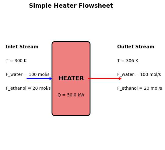
Visualizing a Flowsheet#
A picture is worth a thousand numbers. Let’s create a simple visualization of our heater flowsheet.
import matplotlib.pyplot as plt
import matplotlib.patches as patches

def draw_heater_flowsheet(inlet, outlet, Q):
    """Draw a simple heater flowsheet diagram."""
    fig, ax = plt.subplots(1, 1, figsize=(12, 5))

    # Draw heater box
    heater_box = patches.FancyBboxPatch(
        (0.38, 0.25), 0.24, 0.5,
        boxstyle="round,pad=0.02",
        facecolor='lightcoral',
        edgecolor='black',
        linewidth=2,
    )
    ax.add_patch(heater_box)
    ax.text(0.5, 0.5, 'HEATER', ha='center', va='center', fontsize=14, fontweight='bold')
    ax.text(0.5, 0.38, f'Q = {Q/1000:.1f} kW', ha='center', va='center', fontsize=10)

    # Draw inlet arrow
    ax.annotate('', xy=(0.37, 0.5), xytext=(0.17, 0.5),
                arrowprops=dict(arrowstyle='->', lw=2, color='blue'))
    ax.text(0.02, 0.72, 'Inlet Stream', fontsize=11, fontweight='bold')
    ax.text(0.02, 0.62, f'T = {inlet["T"]:.0f} K', fontsize=10)
    ax.text(0.02, 0.52, f'F_water = {inlet["F_water"]:.0f} mol/s', fontsize=10)
    ax.text(0.02, 0.42, f'F_ethanol = {inlet["F_ethanol"]:.0f} mol/s', fontsize=10)

    # Draw outlet arrow
    ax.annotate('', xy=(0.88, 0.5), xytext=(0.62, 0.5),
                arrowprops=dict(arrowstyle='->', lw=2, color='red'))
    ax.text(0.84, 0.72, 'Outlet Stream', fontsize=11, fontweight='bold')
    ax.text(0.84, 0.62, f'T = {outlet["T"]:.0f} K', fontsize=10)
    ax.text(0.84, 0.52, f'F_water = {outlet["F_water"]:.0f} mol/s', fontsize=10)
    ax.text(0.84, 0.42, f'F_ethanol = {outlet["F_ethanol"]:.0f} mol/s', fontsize=10)

    ax.set_xlim(0, 1)
    ax.set_ylim(0, 1)
    ax.set_aspect('equal')
    ax.axis('off')
    ax.set_title('Simple Heater Flowsheet', fontsize=14, fontweight='bold')

    plt.tight_layout()
    return fig

# Draw the flowsheet
fig = draw_heater_flowsheet(
    inlet={'F_water': 100.0, 'F_ethanol': 20.0, 'T': 300.0},
    outlet={'F_water': 100.0, 'F_ethanol': 20.0, 'T': float(outlet_jax['T'])},
    Q=50000.0
)
Key Concepts Summary#
Concept |
Physical Meaning |
Code Representation |
|---|---|---|
Stream |
Flowing mixture of chemicals |
Dictionary with flows, T, P |
Unit Operation |
Equipment that transforms streams |
Function: |
Flowsheet |
Connected network of equipment |
Sequence of function calls |
Flow rate \(F_i\) |
Amount of species \(i\) passing per second |
|
Temperature \(T\) |
Thermal energy of the stream |
|
Pressure \(P\) |
Force per unit area |
|
Try It Yourself!#
Modify the code below to explore how the heater behaves.
# Exercise 1: What happens if you double the heat duty?
# Try changing Q from 50000 to 100000 and re-run

Q_test = 50000.0  # <-- Change this value!

outlet_test = simple_heater_jax(inlet_jax, jnp.array(Q_test), Cp_jax)
print(f"Heat duty: {Q_test/1000:.1f} kW")
print(f"Outlet temperature: {float(outlet_test['T']):.1f} K")
print(f"Temperature rise: {float(outlet_test['T']) - float(inlet_jax['T']):.1f} K")
Heat duty: 50.0 kW
Outlet temperature: 305.6 K
Temperature rise: 5.6 K
# Exercise 2: What happens if you increase the flow rate?
# More flow means less temperature rise for the same heat duty

F_water_test = 100.0  # <-- Try 200, 500, etc.

inlet_test = {
    'F_water': jnp.array(F_water_test),
    'F_ethanol': jnp.array(20.0),
    'T': jnp.array(300.0),
    'P': jnp.array(101325.0),
}

outlet_test = simple_heater_jax(inlet_test, jnp.array(50000.0), Cp_jax)
print(f"Water flow rate: {F_water_test} mol/s")
print(f"Total flow rate: {F_water_test + 20.0} mol/s")
print(f"Outlet temperature: {float(outlet_test['T']):.1f} K")
print(f"Temperature rise: {float(outlet_test['T']) - 300.0:.1f} K")
Water flow rate: 100.0 mol/s
Total flow rate: 120.0 mol/s
Outlet temperature: 305.6 K
Temperature rise: 5.6 K
End-of-Tutorial Problems#
Problem 1: Stream Properties#
A stream contains:
Methane: 50 mol/s
Ethane: 30 mol/s
Propane: 20 mol/s
Calculate:
a) The total molar flow rate
b) The mole fraction of each component
c) Create this stream using make_stream with T=298 K and P=500000 Pa
# Your solution here

# a) Total molar flow rate
F_total = None  # Calculate this

# b) Mole fractions
y_methane = None  # Calculate this
y_ethane = None
y_propane = None

# c) Create stream with make_stream
# natural_gas = make_stream(...)
Problem 2: Cooler Design#
Modify the simple_heater_jax function to create a simple_cooler_jax function that:
Takes a hot inlet stream and a heat removal rate Q (negative value)
Returns a cooled outlet stream
Test it by cooling a stream from 400 K to approximately 350 K.
# Your solution here

def simple_cooler_jax(inlet, Q, Cp_mixture):
    """Cool a stream by removing heat duty Q (Q should be negative)."""
    # Your code here
    pass
Problem 3: Thinking Question#
Why do we use dictionaries with string keys (like 'F_water') instead of just arrays of numbers?
Think about:
Readability
Error prevention
Flexibility when adding/removing species
Your answer here:
Next Steps#
In the next notebook (00b: What is a Flowsheet? Intermediate), we’ll explore:
The mathematical view: flowsheets as systems of equations
How streams become “shared variables” between units
Degrees of freedom analysis
This will deepen your understanding of what the computer is actually solving when you simulate a flowsheet.