
Single Unit: Energy Balances#
Prerequisites: 00d_single_unit_cstr
Learning Objectives:
Derive the energy balance equation for reactors
Understand heat of reaction and its effect on temperature
Compare isothermal, adiabatic, and specified-duty operation
Implement non-isothermal CSTR calculations
Why Energy Balances Matter#
In the CSTR tutorial, we assumed isothermal operation (constant temperature). In reality:
Exothermic reactions release heat → temperature rises unless we remove heat
Endothermic reactions absorb heat → temperature falls unless we add heat
Temperature affects reaction rate (Arrhenius kinetics)
The energy balance tells us:
How much heat must be added/removed for isothermal operation
What temperature the reactor reaches if adiabatic
How temperature and conversion are coupled
Deriving the Energy Balance#
For a CSTR at steady state:
where:
\(\dot{Q}\) = heat added to the system (W)
\(F_i\) = molar flow rate of species \(i\) (mol/s)
\(\bar{H}_i\) = molar enthalpy of species \(i\) (J/mol)
Simplification with Heat Capacity#
For ideal solutions with constant heat capacity:
After substitution and rearrangement:
where:
\(\xi_j = V \cdot r_j\) = extent of reaction \(j\) (mol/s)
\(\Delta H_{rxn,j}\) = heat of reaction for reaction \(j\) (J/mol)
Heat of Reaction#
The heat of reaction \(\Delta H_{rxn}\) is the enthalpy change when the reaction occurs:
where:
\(\nu_i\) = stoichiometric coefficient (negative for reactants, positive for products)
\(\bar{H}_{f,i}\) = heat of formation of species \(i\)
Sign convention:
\(\Delta H_{rxn} < 0\): Exothermic (releases heat)
\(\Delta H_{rxn} > 0\): Endothermic (absorbs heat)
# Setup
import jax.numpy as jnp
import jax
jax.config.update("jax_enable_x64", True)
import matplotlib.pyplot as plt
import numpy as np

from difflow import CSTR, CSTRParams, make_stream, get_flows, IdealThermo, SpeciesData
WARNING:2026-01-10 21:08:32,758:jax._src.xla_bridge:852: An NVIDIA GPU may be present on this machine, but a CUDA-enabled jaxlib is not installed. Falling back to cpu.
# Example: Exothermic reaction A -> B with ΔH_rxn = -50 kJ/mol

# Define species with heats of formation
species_data = {
    'A': SpeciesData(
        name='A', MW=50.0,
        Cp_coeffs=(50.0, 0, 0, 0),  # J/(mol·K)
        Hvap_coeffs=(30000.0, 0.38, 400.0),
        antoine_coeffs=(10.0, 2000.0, -40.0),
        Hf=0.0,  # Reference: Hf_A = 0
    ),
    'B': SpeciesData(
        name='B', MW=50.0,
        Cp_coeffs=(50.0, 0, 0, 0),
        Hvap_coeffs=(28000.0, 0.38, 380.0),
        antoine_coeffs=(10.0, 1800.0, -40.0),
        Hf=-50000.0,  # ΔH_rxn = Hf_B - Hf_A = -50 kJ/mol (exothermic)
    ),
}
thermo = IdealThermo(species_data)
species_order = ['A', 'B']

# Calculate heat of reaction
dH_rxn = species_data['B'].Hf - species_data['A'].Hf
print(f"Heat of reaction: ΔH_rxn = {dH_rxn/1000:.0f} kJ/mol")
print("This is EXOTHERMIC (releases heat)")
Heat of reaction: ΔH_rxn = -50 kJ/mol
This is EXOTHERMIC (releases heat)
# Rate function with Arrhenius temperature dependence

def rate_fn_arrhenius(C, T, params):
    """
    First-order reaction A -> B with Arrhenius kinetics.

    k = A * exp(-Ea / RT)
    r = k * C_A
    """
    A = params['A']     # Pre-exponential factor, 1/s
    Ea = params['Ea']   # Activation energy, J/mol
    R = 8.314           # Gas constant, J/(mol·K)

    k = A * jnp.exp(-Ea / (R * T))
    r = k * C['A']

    return jnp.array([r])

# Stoichiometry: A -> B
stoich = jnp.array([[-1.0], [1.0]])

# Kinetic parameters
rate_params = {
    'A': jnp.array(1e8),      # 1/s
    'Ea': jnp.array(50000.0), # J/mol
}

# At T = 350 K:
T_test = 350.0
k_test = float(rate_params['A'] * jnp.exp(-rate_params['Ea'] / (8.314 * T_test)))
print(f"At T = {T_test} K: k = {k_test:.4f} /s")
At T = 350.0 K: k = 3.4486 /s
Three Modes of Operation#
1. Isothermal Operation#
Temperature is held constant. The heat duty Q is calculated to maintain T.
2. Adiabatic Operation#
No heat transfer (Q = 0). Temperature changes due to reaction.
3. Specified Heat Duty#
Q is specified. Temperature is calculated.
# Create feed stream
F_A_in = 10.0  # mol/s
T_in = 350.0   # K
Q_vol = 0.1    # m³/s
V = 1.0        # m³

feed = make_stream({'A': F_A_in, 'B': 0.0}, T=T_in, P=101325.0)
# Mode 1: ISOTHERMAL
# We specify the outlet temperature = inlet temperature
# The reactor calculates Q needed

cstr_isothermal_params = CSTRParams(
    V=jnp.array(V),
    rate_fn=rate_fn_arrhenius,
    stoich=stoich,
    rate_params=rate_params,
    species_order=species_order,
    dH_rxn=jnp.array([dH_rxn]),
)

cstr_isothermal = CSTR(cstr_isothermal_params, thermo=thermo, mode='isothermal')
outlet_iso, info_iso = cstr_isothermal(feed, T_spec=T_in, volumetric_flow=Q_vol)

print("MODE 1: ISOTHERMAL")
print("=" * 50)
print(f"Inlet T  = {T_in} K")
print(f"Outlet T = {float(outlet_iso['T']):.1f} K")
print(f"Conversion = {float(info_iso['conversion']['A'])*100:.1f}%")
print(f"Heat duty Q = {float(info_iso['Q'])/1000:.2f} kW")
print(f"\n(Negative Q means heat must be REMOVED - cooling required)")
MODE 1: ISOTHERMAL
==================================================
Inlet T  = 350.0 K
Outlet T = 350.0 K
Conversion = 97.2%
Heat duty Q = -485.91 kW

(Negative Q means heat must be REMOVED - cooling required)
# Mode 2: ADIABATIC
# No heat transfer - temperature changes with reaction

cstr_adiabatic = CSTR(cstr_isothermal_params, thermo=thermo, mode='adiabatic')
outlet_adi, info_adi = cstr_adiabatic(feed, volumetric_flow=Q_vol)

print("MODE 2: ADIABATIC")
print("=" * 50)
print(f"Inlet T  = {T_in} K")
print(f"Outlet T = {float(outlet_adi['T']):.1f} K")
print(f"Conversion = {float(info_adi['conversion']['A'])*100:.1f}%")
print(f"Heat duty Q = {float(info_adi['Q'])/1000:.2f} kW (should be ~0)")
print(f"\nTemperature rise: ΔT = {float(outlet_adi['T']) - T_in:.1f} K")
print(f"(Exothermic reaction heats up the mixture)")
MODE 2: ADIABATIC
==================================================
Inlet T  = 350.0 K
Outlet T = 1350.0 K
Conversion = 100.0%
Heat duty Q = 0.00 kW (should be ~0)

Temperature rise: ΔT = 1000.0 K
(Exothermic reaction heats up the mixture)
# Mode 3: SPECIFIED HEAT DUTY
# We provide some cooling, but not enough for isothermal operation

Q_specified = -15000.0  # W (15 kW cooling)

cstr_specified = CSTR(cstr_isothermal_params, thermo=thermo, mode='specified_duty')
outlet_spec, info_spec = cstr_specified(feed, Q_spec=Q_specified, volumetric_flow=Q_vol)

print("MODE 3: SPECIFIED HEAT DUTY")
print("=" * 50)
print(f"Inlet T  = {T_in} K")
print(f"Outlet T = {float(outlet_spec['T']):.1f} K")
print(f"Conversion = {float(info_spec['conversion']['A'])*100:.1f}%")
print(f"Heat duty Q = {Q_specified/1000:.2f} kW (specified)")
print(f"\nTemperature rise: ΔT = {float(outlet_spec['T']) - T_in:.1f} K")
MODE 3: SPECIFIED HEAT DUTY
==================================================
Inlet T  = 350.0 K
Outlet T = 1320.0 K
Conversion = 100.0%
Heat duty Q = -15.00 kW (specified)

Temperature rise: ΔT = 970.0 K
# Compare all three modes

print("\nCOMPARISON OF OPERATING MODES")
print("=" * 60)
print(f"{'Mode':<20} {'T_out (K)':<12} {'X (%)':<10} {'Q (kW)':<12}")
print("-" * 60)
print(f"{'Isothermal':<20} {float(outlet_iso['T']):<12.1f} {float(info_iso['conversion']['A'])*100:<10.1f} {float(info_iso['Q'])/1000:<12.2f}")
print(f"{'Adiabatic':<20} {float(outlet_adi['T']):<12.1f} {float(info_adi['conversion']['A'])*100:<10.1f} {float(info_adi['Q'])/1000:<12.2f}")
print(f"{'Specified Q=-15kW':<20} {float(outlet_spec['T']):<12.1f} {float(info_spec['conversion']['A'])*100:<10.1f} {Q_specified/1000:<12.2f}")
COMPARISON OF OPERATING MODES
============================================================
Mode                 T_out (K)    X (%)      Q (kW)
------------------------------------------------------------
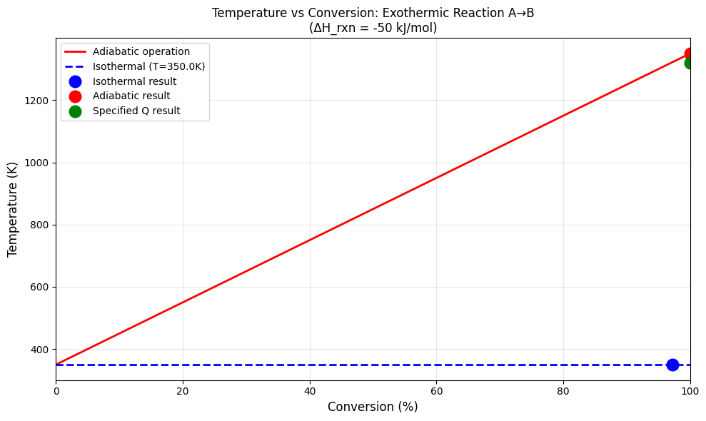
Isothermal           350.0        97.2       -485.91
Adiabatic            1350.0       100.0      0.00
Specified Q=-15kW    1320.0       100.0      -15.00
Visualizing the Energy Balance#
# Plot temperature vs conversion for adiabatic operation

# Adiabatic temperature rise: ΔT = -ξ·ΔH_rxn / (F·Cp)
# where ξ = F_A_in · X is the extent of reaction

X_range = np.linspace(0, 0.99, 100)
Cp_avg = 50.0  # J/(mol·K)
F_total = F_A_in  # mol/s

# Adiabatic temperature: T = T_in + (-ΔH_rxn)·X·F_A_in / (F_total·Cp)
T_adiabatic = T_in + (-dH_rxn) * X_range * F_A_in / (F_total * Cp_avg)

fig, ax = plt.subplots(figsize=(10, 6))

# Adiabatic line
ax.plot(X_range * 100, T_adiabatic, 'r-', linewidth=2, label='Adiabatic operation')

# Isothermal line
ax.axhline(y=T_in, color='b', linestyle='--', linewidth=2, label=f'Isothermal (T={T_in}K)')

# Mark operating points
ax.plot(float(info_iso['conversion']['A'])*100, float(outlet_iso['T']), 'bo', markersize=12, label='Isothermal result')
ax.plot(float(info_adi['conversion']['A'])*100, float(outlet_adi['T']), 'ro', markersize=12, label='Adiabatic result')
ax.plot(float(info_spec['conversion']['A'])*100, float(outlet_spec['T']), 'go', markersize=12, label='Specified Q result')

ax.set_xlabel('Conversion (%)', fontsize=12)
ax.set_ylabel('Temperature (K)', fontsize=12)
ax.set_title('Temperature vs Conversion: Exothermic Reaction A→B\n(ΔH_rxn = -50 kJ/mol)', fontsize=12)
ax.legend(loc='best')
ax.grid(True, alpha=0.3)
ax.set_xlim(0, 100)

plt.tight_layout()
The Raw Equations#
Let’s implement the energy balance from scratch to see what difflow is doing.
def cstr_with_energy_balance_raw(F_in, T_in, V, Q_vol, k_params, dH_rxn, Cp, mode='isothermal', Q_spec=None, T_spec=None):
    """
    Solve CSTR with energy balance from first principles.

    Equations:
        Mass: F_A_out = F_A_in - V·r(C_A, T)
        Energy: Q = F_total·Cp·(T_out - T_in) + ξ·ΔH_rxn

    Mode:
        'isothermal': T_out = T_in, solve for Q
        'adiabatic': Q = 0, solve for T_out
        'specified_duty': Q given, solve for T_out
    """
    F_A_in = F_in[0]
    A, Ea = k_params['A'], k_params['Ea']
    R = 8.314

    if mode == 'isothermal':
        T_out = T_spec if T_spec else T_in

        # Solve mass balance at T_out
        k = A * np.exp(-Ea / (R * T_out))
        tau = V / Q_vol
        C_A_in = F_A_in / Q_vol

        # For first-order: C_A = C_A_in / (1 + k·τ)
        C_A_out = C_A_in / (1 + k * tau)
        F_A_out = C_A_out * Q_vol

        # Extent of reaction
        xi = F_A_in - F_A_out  # mol/s converted

        # Energy balance: Q = F·Cp·ΔT + ξ·ΔH_rxn
        # For isothermal, ΔT = 0
        Q = xi * dH_rxn

        return F_A_out, T_out, Q

    elif mode == 'adiabatic':
        # Need to solve coupled mass and energy balance
        # Iterate to find T_out

        T_out = T_in  # Initial guess
        F_total = F_A_in

        for _ in range(100):
            k = A * np.exp(-Ea / (R * T_out))
            tau = V / Q_vol
            C_A_in = F_A_in / Q_vol
            C_A_out = C_A_in / (1 + k * tau)
            F_A_out = C_A_out * Q_vol
            xi = F_A_in - F_A_out

            # Adiabatic: Q = 0, so F·Cp·(T_out - T_in) = -ξ·ΔH_rxn
            T_out_new = T_in + (-dH_rxn) * xi / (F_total * Cp)

            if abs(T_out_new - T_out) < 1e-6:
                break
            T_out = 0.5 * T_out + 0.5 * T_out_new  # Damped update

        conversion = (F_A_in - F_A_out) / F_A_in
        return F_A_out, T_out, 0.0, conversion

# Test ISOTHERMAL mode
F_A_out_raw, T_out_raw, Q_raw = cstr_with_energy_balance_raw(
    F_in=[F_A_in], T_in=T_in, V=V, Q_vol=Q_vol,
    k_params={'A': float(rate_params['A']), 'Ea': float(rate_params['Ea'])},
    dH_rxn=dH_rxn, Cp=50.0, mode='isothermal'
)

print("Raw Implementation vs difflow (Isothermal)")
print("=" * 50)
print(f"{'Quantity':<20} {'Raw':<15} {'difflow':<15}")
print("-" * 50)
print(f"{'F_A_out (mol/s)':<20} {F_A_out_raw:<15.4f} {float(get_flows(outlet_iso)['A']):<15.4f}")
print(f"{'T_out (K)':<20} {T_out_raw:<15.1f} {float(outlet_iso['T']):<15.1f}")
print(f"{'Q (kW)':<20} {Q_raw/1000:<15.2f} {float(info_iso['Q'])/1000:<15.2f}")

# Test ADIABATIC mode
F_A_out_raw_adi, T_out_raw_adi, Q_raw_adi, X_raw_adi = cstr_with_energy_balance_raw(
    F_in=[F_A_in], T_in=T_in, V=V, Q_vol=Q_vol,
    k_params={'A': float(rate_params['A']), 'Ea': float(rate_params['Ea'])},
    dH_rxn=dH_rxn, Cp=50.0, mode='adiabatic'
)

print("\n\nRaw Implementation vs difflow (Adiabatic)")
print("=" * 50)
print(f"{'Quantity':<20} {'Raw':<15} {'difflow':<15}")
print("-" * 50)
print(f"{'F_A_out (mol/s)':<20} {F_A_out_raw_adi:<15.4f} {float(get_flows(outlet_adi)['A']):<15.4f}")
print(f"{'T_out (K)':<20} {T_out_raw_adi:<15.1f} {float(outlet_adi['T']):<15.1f}")
print(f"{'Conversion (%)':<20} {X_raw_adi*100:<15.1f} {float(info_adi['conversion']['A'])*100:<15.1f}")

print("\n✓ Both implementations agree!")
Raw Implementation vs difflow (Isothermal)
==================================================
Quantity             Raw             difflow
--------------------------------------------------
F_A_out (mol/s)      0.2818          0.2818
T_out (K)            350.0           350.0
Q (kW)               -485.91         -485.91


Raw Implementation vs difflow (Adiabatic)
==================================================
Quantity             Raw             difflow
--------------------------------------------------
F_A_out (mol/s)      0.0000          0.0000
T_out (K)            1350.0          1350.0
Conversion (%)       100.0           100.0

✓ Both implementations agree!
Try It Yourself!#
Exercise 1: Endothermic Reaction#
Change the heat of reaction to +30 kJ/mol (endothermic). What happens to the adiabatic temperature? Does conversion go up or down?
# Your solution here
Exercise 2: Multiple Steady States#
Exothermic reactions in adiabatic CSTRs can have multiple steady states. Try varying the inlet temperature from 300K to 400K and plot the outlet temperature. Do you see any jumps?
# Your solution here
End-of-Tutorial Problems#
Problem 1: Heat Duty Calculation#
For the reaction A → B with ΔH_rxn = -80 kJ/mol:
Feed: 20 mol/s pure A at 400 K
Conversion: 60%
Outlet temperature: 400 K (isothermal)
Calculate the heat duty required (in kW).
Problem 2: Adiabatic Temperature Rise#
For the same reaction, if operated adiabatically with Cp = 100 J/(mol·K), what is the outlet temperature at 60% conversion?
Problem 3: Cooling Jacket Design#
If the cooling water can remove heat at a rate of -50 kW, what is the maximum conversion achievable while keeping T_out ≤ 420 K?
Key Takeaways#
Energy balance: \(Q = F \cdot C_p \cdot \Delta T + \xi \cdot \Delta H_{rxn}\)
Exothermic reactions (\(\Delta H_{rxn} < 0\)) release heat → temperature rises in adiabatic operation
Three operating modes: Isothermal, adiabatic, specified duty
Temperature affects rate: Higher T → faster reaction (Arrhenius)
Coupled equations: Mass and energy balances must be solved together
Next Steps#
In the next notebook (00f: Single Unit - The PFR), we’ll explore:
The plug flow reactor (PFR) design equation
Why it’s an ODE instead of algebraic
Comparison of CSTR vs PFR performance