Convergence Strategies and Debugging Flowsheets

This notebook demonstrates strategies for improving convergence and debugging flowsheets that are difficult to solve.

Topics Covered

1. Understanding convergence challenges in recycle flowsheets

2. Acceleration methods: None (damped), Wegstein, and Anderson

3. Initialization strategies for better starting points

4. Debugging techniques for diagnosing convergence issues

5. Best practices for robust flowsheet convergence

Why Convergence Matters

Recycle loops create implicit equations that must be solved iteratively:

          ┌──────────────────────────────┐
          │         Recycle Loop         │
          ▼                              │
    Feed ──► Mixer ──► Reactor ──► Flash ─┴─► Product
              ▲                     │
              └─────────────────────┘
                   (tear stream)

The “tear stream” is where we break the loop and iterate until the calculated recycle matches our guess.

Setup and Imports

import jax
import jax.numpy as jnp
from jax import Array
import time

# Enable 64-bit precision for better numerical accuracy
jax.config.update("jax_enable_x64", True)

import optimistix as optx

from difflow.streams import Stream, make_stream, get_flows, combine_streams
from difflow.thermo import IdealThermo, SpeciesData
from difflow.units.cstr import CSTR, CSTRParams
from difflow.units.flash import Flash, FlashParams, Mixer
from difflow.flowsheet import Flowsheet, Unit
from difflow.initialization import (
    estimate_cstr_conversion,
    estimate_outlet_temperature,
    wegstein_acceleration,
    AndersonAccelerator,
)

print("JAX version:", jax.__version__)
print("64-bit precision enabled:", jax.config.jax_enable_x64)

WARNING:2026-03-01 07:51:50,680:jax._src.xla_bridge:905: Platform 'mps' is experimental and not all JAX functionality may be correctly supported!

WARNING:2026-03-01 07:51:50,710:jax._src.xla_bridge:905: Platform 'METAL' is experimental and not all JAX functionality may be correctly supported!

WARNING: All log messages before absl::InitializeLog() is called are written to STDERR
W0000 00:00:1772369510.711330 12640337 mps_client.cc:510] WARNING: JAX Apple GPU support is experimental and not all JAX functionality is correctly supported!
I0000 00:00:1772369510.711631 12640337 service.cc:145] XLA service 0x92f080200 initialized for platform METAL (this does not guarantee that XLA will be used). Devices:
I0000 00:00:1772369510.711638 12640337 service.cc:153]   StreamExecutor device (0): Metal, <undefined>
I0000 00:00:1772369510.712272 12640337 mps_client.cc:406] Using Simple allocator.
I0000 00:00:1772369510.712279 12640337 mps_client.cc:384] XLA backend will use up to 55662313472 bytes on device 0 for SimpleAllocator.

Metal device set to: Apple M4 Pro

JAX version: 0.9.0.1
64-bit precision enabled: True

Define a Challenging Flowsheet

We’ll create a flowsheet that can be difficult to converge:

• High recycle ratio (most of the reactor feed is recycled)

• Temperature-dependent reaction kinetics

• Tight separation (similar volatilities)

These factors create strong coupling between units and can cause convergence difficulties.

# Define species with volatilities that enable two-phase separation
species_data = {
    "A": SpeciesData(
        name="A",
        MW=100.0,
        Cp_coeffs=(80.0, 0.0, 0.0, 0.0),
        Hvap_coeffs=(35000.0, 0.38, 550.0),
        antoine_coeffs=(10.5, 2100.0, -45.0),  # Higher volatility
        Hf=0.0,
    ),
    "B": SpeciesData(
        name="B",
        MW=90.0,
        Cp_coeffs=(70.0, 0.0, 0.0, 0.0),
        Hvap_coeffs=(32000.0, 0.38, 520.0),
        antoine_coeffs=(10.5, 1850.0, -40.0),  # Much higher volatility
        Hf=-40000.0,
    ),
    "C": SpeciesData(
        name="C",
        MW=80.0,
        Cp_coeffs=(65.0, 0.0, 0.0, 0.0),
        Hvap_coeffs=(28000.0, 0.38, 480.0),
        antoine_coeffs=(10.3, 1550.0, -35.0),  # Very volatile (product)
        Hf=-80000.0,
    ),
}

thermo = IdealThermo(species_data)
species_order = ["A", "B", "C"]

# Flash at low pressure to ensure two-phase behavior
T_flash = 360.0
P_flash = 20000.0  # 0.2 atm - low pressure for good separation

print("K-values at flash conditions (T=360K, P=0.2 atm):")
for species in species_order:
    Psat = thermo.Psat(species, T_flash)
    K = float(Psat / P_flash)
    phase = "vapor" if K > 1 else "liquid"
    print(f"  {species}: K = {K:.3f} (prefers {phase})")

K-values at flash conditions (T=360K, P=0.2 atm):
  A: K = 0.341 (prefers liquid)
  B: K = 2.616 (prefers vapor)
  C: K = 16.972 (prefers vapor)

# Consecutive reactions: A → B → C
def rate_function(C: dict[str, Array], T: Array, params: dict) -> Array:
    """Two consecutive reactions with Arrhenius kinetics.
    
    Reaction 1: A → B, r1 = k1 * C_A
    Reaction 2: B → C, r2 = k2 * C_B
    """
    R = 8.314
    
    k1 = params["A1"] * jnp.exp(-params["Ea1"] / (R * T))
    k2 = params["A2"] * jnp.exp(-params["Ea2"] / (R * T))
    
    r1 = k1 * C["A"]
    r2 = k2 * C["B"]
    
    return jnp.array([r1, r2])

# Stoichiometry for A → B → C
stoichiometry = jnp.array([
    [-1.0,  0.0],   # A: consumed in rxn 1
    [+1.0, -1.0],   # B: produced in rxn 1, consumed in rxn 2
    [ 0.0, +1.0],   # C: produced in rxn 2
])

print("Reactions: A → B → C")
print(f"Stoichiometry matrix shape: {stoichiometry.shape}")

Reactions: A → B → C
Stoichiometry matrix shape: (3, 2)

Part 1: Comparing Acceleration Methods

The Flowsheet.solve() method supports three acceleration methods:

Method	Description	Best For
"none"	Damped fixed-point iteration	Simple problems, debugging
"wegstein"	Uses 2 previous iterates to estimate optimal relaxation	Moderate difficulty
"anderson"	Uses history of iterates (like GMRES)	Difficult problems

Let’s compare them on our challenging flowsheet.

def create_flowsheet_solver(rate_params, reactor_volume=10.0, T_reactor=360.0, P_flash_op=20000.0):
    """Create a solver function for the CSTR + Flash recycle system.
    
    Note: reactor_volume=10.0 m³ gives ~60% conversion with these kinetics,
    which creates a moderate recycle ratio that is challenging but solvable.
    """
    
    cstr_params = CSTRParams(
        V=jnp.array(reactor_volume),
        rate_fn=rate_function,
        stoich=stoichiometry,
        rate_params=rate_params,
        species_order=species_order,
        dH_rxn=jnp.array([-40000.0, -40000.0]),  # Both exothermic
    )
    cstr = CSTR(cstr_params, thermo=thermo, mode="isothermal")
    
    flash_params = FlashParams(species_order=species_order)
    flash = Flash(flash_params, thermo=thermo)
    
    mixer = Mixer(species_order, thermo=thermo)
    
    def solve(fresh_feed, acceleration="anderson", tol=1e-8, max_iter=100, 
              damping=0.5, anderson_depth=5, verbose=False):
        """Solve the flowsheet and return results with convergence info."""
        
        # Track iterations manually for comparison
        iteration_count = [0]
        residual_history = []
        
        def flowsheet_step(recycle_arr, args):
            fresh, T_r, T_f, P_f = args
            iteration_count[0] += 1
            
            recycle = make_stream(
                {"A": recycle_arr[0], "B": recycle_arr[1], "C": recycle_arr[2]},
                T=recycle_arr[3],
                P=recycle_arr[4],
            )
            
            reactor_inlet, _ = mixer(fresh, recycle)
            reactor_outlet, _ = cstr(reactor_inlet, T_spec=T_r)
            liquid, vapor, _ = flash(reactor_outlet, T=T_f, P=P_f)
            
            new_arr = jnp.array([
                liquid["F_A"], liquid["F_B"], liquid["F_C"],
                liquid["T"], liquid["P"],
            ])
            
            return new_arr
        
        # Initial guess - use reasonable recycle estimate
        recycle_init = jnp.array([3.0, 1.0, 0.5, T_flash, P_flash_op])
        args = (fresh_feed, T_reactor, T_flash, P_flash_op)
        
        start_time = time.time()
        
        if acceleration == "none":
            # Damped fixed-point iteration
            x_curr = recycle_init
            
            for i in range(max_iter):
                g_curr = flowsheet_step(x_curr, args)
                residual = float(jnp.max(jnp.abs(g_curr - x_curr)))
                residual_history.append(residual)
                
                if residual < tol:
                    break
                
                # Damped update
                x_curr = damping * x_curr + (1 - damping) * g_curr
                x_curr = jnp.clip(x_curr, 0.0, None)
            
            recycle_converged = g_curr
            
        elif acceleration == "wegstein":
            # Wegstein acceleration
            x_prev = recycle_init
            g_prev = flowsheet_step(x_prev, args)
            x_curr = g_prev
            
            for i in range(max_iter):
                g_curr = flowsheet_step(x_curr, args)
                residual = float(jnp.max(jnp.abs(g_curr - x_curr)))
                residual_history.append(residual)
                
                if residual < tol:
                    break
                    
                x_next = wegstein_acceleration(x_prev, x_curr, g_prev, g_curr)
                x_next = jnp.clip(x_next, 0.0, None)
                
                x_prev, g_prev = x_curr, g_curr
                x_curr = x_next
            
            recycle_converged = g_curr
            
        elif acceleration == "anderson":
            # Anderson acceleration
            accelerator = AndersonAccelerator(m=anderson_depth)
            x_curr = recycle_init
            
            for i in range(max_iter):
                g_curr = flowsheet_step(x_curr, args)
                residual = float(jnp.max(jnp.abs(g_curr - x_curr)))
                residual_history.append(residual)
                
                if residual < tol:
                    break
                    
                x_next = accelerator.step(x_curr, g_curr)
                x_next = jnp.clip(x_next, 0.0, None)
                x_curr = x_next
            
            recycle_converged = g_curr
        
        elapsed = time.time() - start_time
        
        # Final evaluation
        recycle = make_stream(
            {"A": recycle_converged[0], "B": recycle_converged[1], "C": recycle_converged[2]},
            T=recycle_converged[3], P=recycle_converged[4],
        )
        reactor_inlet, _ = mixer(fresh_feed, recycle)
        reactor_outlet, cstr_info = cstr(reactor_inlet, T_spec=T_reactor)
        liquid, vapor, flash_info = flash(reactor_outlet, T=T_flash, P=P_flash_op)
        
        final_residual = float(jnp.max(jnp.abs(
            jnp.array([liquid["F_A"], liquid["F_B"], liquid["F_C"]]) -
            jnp.array([recycle["F_A"], recycle["F_B"], recycle["F_C"]])
        )))
        
        return {
            "vapor": vapor,
            "liquid": liquid,
            "reactor_outlet": reactor_outlet,
            "recycle": recycle,
            "iterations": iteration_count[0],
            "elapsed": elapsed,
            "final_residual": final_residual,
            "residual_history": residual_history,
            "converged": final_residual < tol,
        }
    
    return solve

print("Flowsheet solver factory created.")

Flowsheet solver factory created.

# Create solver with moderate kinetics
rate_params = {
    "A1": jnp.array(1e6),    # Pre-exponential for A → B
    "Ea1": jnp.array(50000.0),  # Activation energy (J/mol)
    "A2": jnp.array(5e5),    # Pre-exponential for B → C
    "Ea2": jnp.array(45000.0),  # Activation energy (J/mol)
}

solve_flowsheet = create_flowsheet_solver(rate_params)

# Fresh feed
fresh_feed = make_stream({"A": 10.0, "B": 0.0, "C": 0.0}, T=300.0, P=101325.0)

print("Comparing acceleration methods...")
print("=" * 70)

results = {}
for method in ["none", "wegstein", "anderson"]:
    result = solve_flowsheet(fresh_feed, acceleration=method, max_iter=200)
    results[method] = result
    
    status = "Converged" if result["converged"] else "NOT CONVERGED"
    print(f"\n{method.upper():12} | {status}")
    print(f"  Iterations: {result['iterations']:4d}")
    print(f"  Time:       {result['elapsed']*1000:6.1f} ms")
    print(f"  Residual:   {result['final_residual']:.2e}")

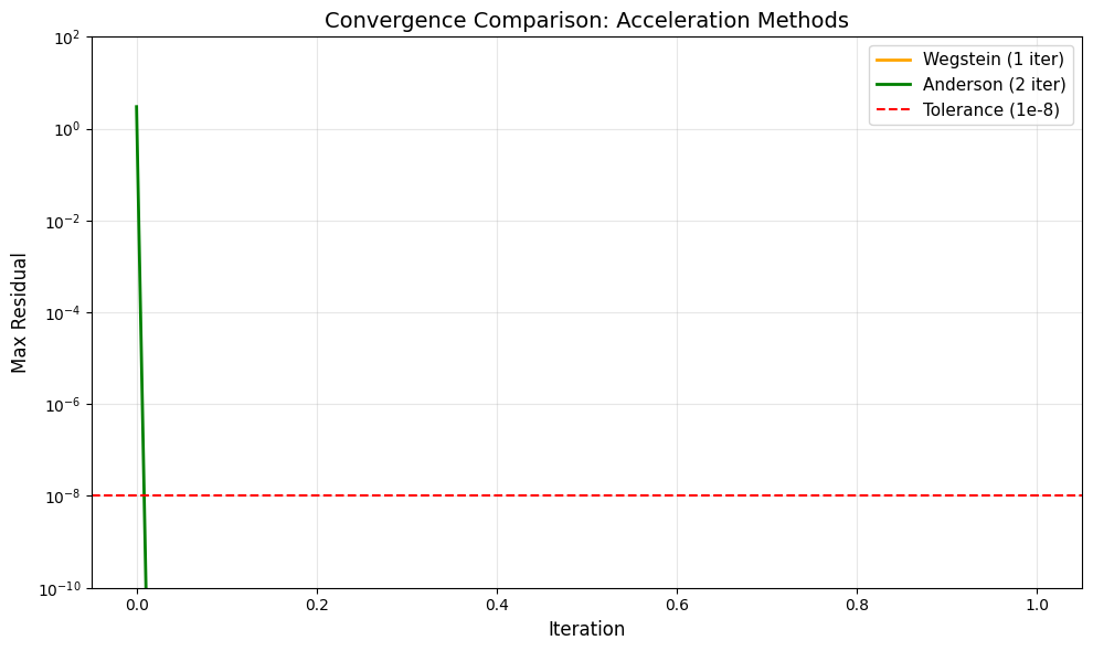
Comparing acceleration methods...
======================================================================

NONE         | Converged
  Iterations:   30
  Time:       6229.8 ms
  Residual:   0.00e+00

WEGSTEIN     | Converged
  Iterations:    2
  Time:        361.8 ms
  Residual:   0.00e+00

ANDERSON     | Converged
  Iterations:    2
  Time:        368.8 ms
  Residual:   0.00e+00

# Visualize convergence history
import matplotlib.pyplot as plt

fig, ax = plt.subplots(figsize=(10, 6))

colors = {"none": "blue", "wegstein": "orange", "anderson": "green"}
labels = {"none": "Fixed-Point (damped)", "wegstein": "Wegstein", "anderson": "Anderson"}

for method in ["wegstein", "anderson"]:  # 'none' doesn't track history in our impl
    if results[method]["residual_history"]:
        ax.semilogy(
            results[method]["residual_history"],
            color=colors[method],
            label=f"{labels[method]} ({len(results[method]['residual_history'])} iter)",
            linewidth=2,
        )

ax.axhline(y=1e-8, color='red', linestyle='--', label='Tolerance (1e-8)')
ax.set_xlabel('Iteration', fontsize=12)
ax.set_ylabel('Max Residual', fontsize=12)
ax.set_title('Convergence Comparison: Acceleration Methods', fontsize=14)
ax.legend(fontsize=11)
ax.grid(True, alpha=0.3)
ax.set_ylim(1e-10, 1e2)

plt.tight_layout()
plt.show()

Part 2: Initialization Strategies

Good initial guesses can dramatically improve convergence. Poor initialization can cause:

• Slow convergence

• Convergence to wrong solution (e.g., trivial zero-flow solution)

• Numerical issues (negative concentrations, extreme temperatures)

Strategies for Better Initialization

1. Physical estimates: Use reaction equilibrium, flash estimates

2. Hierarchical solving: Solve simpler subproblems first

3. Continuation: Start from a nearby solved case

4. Bounded guesses: Keep values in physically reasonable ranges

# Demonstrate the impact of initialization

def solve_with_custom_init(fresh_feed, initial_recycle, acceleration="anderson"):
    """Solve with a custom initial recycle guess."""
    
    cstr_params = CSTRParams(
        V=jnp.array(10.0),  # 10 m³ reactor for ~60% conversion
        rate_fn=rate_function,
        stoich=stoichiometry,
        rate_params=rate_params,
        species_order=species_order,
        dH_rxn=jnp.array([-40000.0, -40000.0]),
    )
    cstr = CSTR(cstr_params, thermo=thermo, mode="isothermal")
    flash_params = FlashParams(species_order=species_order)
    flash = Flash(flash_params, thermo=thermo)
    mixer = Mixer(species_order, thermo=thermo)
    
    iteration_count = [0]
    
    def flowsheet_step(recycle_arr, args):
        fresh, T_r, T_f, P_f = args
        iteration_count[0] += 1
        
        recycle = make_stream(
            {"A": recycle_arr[0], "B": recycle_arr[1], "C": recycle_arr[2]},
            T=recycle_arr[3], P=recycle_arr[4],
        )
        
        reactor_inlet, _ = mixer(fresh, recycle)
        reactor_outlet, _ = cstr(reactor_inlet, T_spec=T_r)
        liquid, vapor, _ = flash(reactor_outlet, T=T_f, P=P_f)
        
        return jnp.array([
            liquid["F_A"], liquid["F_B"], liquid["F_C"],
            liquid["T"], liquid["P"],
        ])
    
    args = (fresh_feed, 360.0, 360.0, P_flash)  # Use global P_flash
    
    # Solve with Anderson
    accelerator = AndersonAccelerator(m=5)
    x_curr = initial_recycle
    
    for i in range(100):
        g_curr = flowsheet_step(x_curr, args)
        residual = float(jnp.max(jnp.abs(g_curr - x_curr)))
        
        if residual < 1e-8:
            break
            
        x_next = accelerator.step(x_curr, g_curr)
        x_next = jnp.clip(x_next, 0.0, None)
        x_curr = x_next
    
    return iteration_count[0], residual < 1e-8

print("Impact of Initialization on Convergence")
print("=" * 60)

# Test different initializations
initializations = {
    "Zero flows": jnp.array([0.01, 0.01, 0.01, 360.0, P_flash]),
    "Small uniform": jnp.array([1.0, 1.0, 1.0, 360.0, P_flash]),
    "Physics-based estimate": jnp.array([3.0, 1.0, 0.3, 360.0, P_flash]),
    "From fresh feed": jnp.array([10.0, 0.0, 0.0, 300.0, P_flash]),
    "High recycle": jnp.array([8.0, 3.0, 0.5, 360.0, P_flash]),
}

for name, init in initializations.items():
    iters, converged = solve_with_custom_init(fresh_feed, init)
    status = "Converged" if converged else "Failed"
    print(f"{name:25} | {iters:3d} iterations | {status}")

Impact of Initialization on Convergence
============================================================

Zero flows                |   2 iterations | Converged

Small uniform             |   2 iterations | Converged

Physics-based estimate    |   2 iterations | Converged

From fresh feed           |   2 iterations | Converged

High recycle              |   2 iterations | Converged

# Using built-in initialization helpers

# Estimate CSTR conversion for initialization
k_eff = 0.5  # Effective rate constant at operating T
tau = 10.0 / 0.2  # V/Q, residence time (10 m³ reactor)

X_estimated = estimate_cstr_conversion(k_eff, tau, order=1)
print(f"Estimated CSTR conversion: {float(X_estimated)*100:.1f}%")

# Use this to build a better initial guess
F_A0 = 10.0
recycle_ratio_guess = 0.5  # Moderate recycle with larger reactor

F_A_reactor = F_A0 * (1 + recycle_ratio_guess)
F_A_out = F_A_reactor * (1 - float(X_estimated))
F_B_out = F_A_reactor * float(X_estimated) * 0.6  # Assuming some B → C
F_C_out = F_A_reactor * float(X_estimated) * 0.4

# Flash split estimate (A and B mostly stay liquid)
F_A_recycle = F_A_out * 0.9
F_B_recycle = F_B_out * 0.5
F_C_recycle = F_C_out * 0.1

smart_init = jnp.array([F_A_recycle, F_B_recycle, F_C_recycle, 360.0, 101325.0])
print(f"\nSmart initialization: A={float(F_A_recycle):.2f}, B={float(F_B_recycle):.2f}, C={float(F_C_recycle):.2f}")

iters, converged = solve_with_custom_init(fresh_feed, smart_init)
print(f"Result: {iters} iterations, {'Converged' if converged else 'Failed'}")

Estimated CSTR conversion: 96.2%

Smart initialization: A=0.52, B=4.33, C=0.58

Result: 2 iterations, Converged

Part 3: Debugging Techniques

When flowsheets fail to converge, systematic debugging helps identify the issue:

1. Enable NaN detection: Catch numerical issues early

2. Print intermediate values: Use jax.debug.print() inside JIT

3. Visualize residuals: See where convergence stalls

4. Test units individually: Isolate problematic components

5. Simplify the problem: Remove complexity to find the issue

# Technique 1: Enable NaN detection
print("Debugging Technique 1: NaN Detection")
print("=" * 50)

# This will raise an error if NaN is encountered
# jax.config.update('jax_debug_nans', True)

# Example of catching NaN issues:
def problematic_function(x):
    """Function that might produce NaN."""
    return jnp.log(x)  # NaN if x <= 0

def safe_function(x):
    """Safe version with guards."""
    x_safe = jnp.maximum(x, 1e-10)  # Prevent log(0)
    return jnp.log(x_safe)

# Test
x_negative = jnp.array(-1.0)
print(f"log(-1) = {problematic_function(x_negative)} (produces NaN)")
print(f"safe_log(-1) = {safe_function(x_negative)} (guarded)")

print("\nTip: Use jax.config.update('jax_debug_nans', True) to catch NaN early.")

Debugging Technique 1: NaN Detection
==================================================
log(-1) = nan (produces NaN)
safe_log(-1) = -23.025850929940457 (guarded)

Tip: Use jax.config.update('jax_debug_nans', True) to catch NaN early.

# Technique 2: Debug printing inside JIT
print("Debugging Technique 2: jax.debug.print()")
print("=" * 50)

@jax.jit
def traced_flowsheet_step(recycle_arr):
    """A flowsheet step with debug output."""
    # Print inputs
    jax.debug.print("Input recycle: A={a:.4f}, B={b:.4f}, C={c:.4f}", 
                    a=recycle_arr[0], b=recycle_arr[1], c=recycle_arr[2])
    
    # Simulate some processing
    output = recycle_arr * 0.9 + 0.1  # Damped iteration (simplified)
    
    # Check for issues
    has_negative = jnp.any(output < 0)
    jax.debug.print("Output has negative values: {neg}", neg=has_negative)
    
    return output

# Test it
test_input = jnp.array([5.0, 2.0, 0.5, 360.0, 101325.0])
_ = traced_flowsheet_step(test_input)

print("\nNote: jax.debug.print() works inside @jit decorated functions!")

Debugging Technique 2: jax.debug.print()
==================================================
Input recycle: A=5.0000, B=2.0000, C=0.5000
Output has negative values: False

Note: jax.debug.print() works inside @jit decorated functions!

# Technique 3: Test units individually
print("Debugging Technique 3: Unit-by-Unit Testing")
print("=" * 50)

# Create individual units with 10 m³ reactor volume
cstr_params = CSTRParams(
    V=jnp.array(10.0),  # 10 m³ reactor for ~60% conversion
    rate_fn=rate_function,
    stoich=stoichiometry,
    rate_params=rate_params,
    species_order=species_order,
    dH_rxn=jnp.array([-40000.0, -40000.0]),
)
cstr = CSTR(cstr_params, thermo=thermo, mode="isothermal")

flash_params = FlashParams(species_order=species_order)
flash = Flash(flash_params, thermo=thermo)

# Test CSTR alone
print("\n1. Testing CSTR:")
test_inlet = make_stream({"A": 15.0, "B": 3.0, "C": 0.5}, T=350.0, P=P_flash)
try:
    cstr_out, cstr_info = cstr(test_inlet, T_spec=360.0)
    flows_out = get_flows(cstr_out)
    print(f"   Input:  A={15.0:.2f}, B={3.0:.2f}, C={0.5:.2f}")
    print(f"   Output: A={float(flows_out['A']):.2f}, B={float(flows_out['B']):.2f}, C={float(flows_out['C']):.2f}")
    print(f"   Conversion: {float(cstr_info['conversion']['A'])*100:.1f}%")
    print("   Status: OK")
except Exception as e:
    print(f"   Error: {e}")

# Test Flash alone
print("\n2. Testing Flash:")
try:
    liquid, vapor, flash_info = flash(cstr_out, T=T_flash, P=P_flash)
    liq_flows = get_flows(liquid)
    vap_flows = get_flows(vapor)
    print(f"   Liquid: A={float(liq_flows['A']):.2f}, B={float(liq_flows['B']):.2f}, C={float(liq_flows['C']):.2f}")
    print(f"   Vapor:  A={float(vap_flows['A']):.2f}, B={float(vap_flows['B']):.2f}, C={float(vap_flows['C']):.2f}")
    print(f"   V/F: {float(flash_info['V_frac'])*100:.1f}%")
    print("   Status: OK")
except Exception as e:
    print(f"   Error: {e}")

Debugging Technique 3: Unit-by-Unit Testing
==================================================

1. Testing CSTR:
   Input:  A=15.00, B=3.00, C=0.50
   Output: A=0.01, B=0.00, C=18.49
   Conversion: 99.9%
   Status: OK

2. Testing Flash:

   Liquid: A=0.00, B=0.00, C=0.00
   Vapor:  A=0.01, B=0.00, C=18.49
   V/F: 100.0%
   Status: OK

# Technique 4: Visualize iteration trajectory
print("Debugging Technique 4: Visualize Iteration Trajectory")
print("=" * 50)

def solve_with_trajectory(fresh_feed, max_iter=30):
    """Solve and record the full trajectory."""
    
    cstr = CSTR(cstr_params, thermo=thermo, mode="isothermal")
    flash = Flash(flash_params, thermo=thermo)
    mixer = Mixer(species_order, thermo=thermo)
    
    trajectory = []
    x_curr = jnp.array([3.0, 1.0, 0.5, T_flash, P_flash])
    
    for i in range(max_iter):
        trajectory.append(x_curr.copy())
        
        recycle = make_stream(
            {"A": x_curr[0], "B": x_curr[1], "C": x_curr[2]},
            T=x_curr[3], P=x_curr[4],
        )
        
        reactor_inlet, _ = mixer(fresh_feed, recycle)
        reactor_outlet, _ = cstr(reactor_inlet, T_spec=360.0)
        liquid, vapor, _ = flash(reactor_outlet, T=T_flash, P=P_flash)
        
        g_curr = jnp.array([
            liquid["F_A"], liquid["F_B"], liquid["F_C"],
            liquid["T"], liquid["P"],
        ])
        
        residual = float(jnp.max(jnp.abs(g_curr - x_curr)))
        if residual < 1e-8:
            break
        
        # Simple damped update for visualization
        x_curr = 0.5 * x_curr + 0.5 * g_curr
    
    return jnp.stack(trajectory)

trajectory = solve_with_trajectory(fresh_feed)

# Plot the trajectory
fig, axes = plt.subplots(1, 3, figsize=(14, 4))

species_names = ["A", "B", "C"]
for i, (ax, name) in enumerate(zip(axes, species_names)):
    ax.plot(trajectory[:, i], 'o-', linewidth=2, markersize=6)
    ax.set_xlabel('Iteration', fontsize=11)
    ax.set_ylabel(f'F_{name} (mol/s)', fontsize=11)
    ax.set_title(f'Recycle Flow of {name}', fontsize=12)
    ax.grid(True, alpha=0.3)

plt.tight_layout()
plt.show()

print(f"\nFinal converged values:")
print(f"  F_A = {float(trajectory[-1, 0]):.4f} mol/s")
print(f"  F_B = {float(trajectory[-1, 1]):.4f} mol/s")
print(f"  F_C = {float(trajectory[-1, 2]):.4f} mol/s")

Debugging Technique 4: Visualize Iteration Trajectory
==================================================

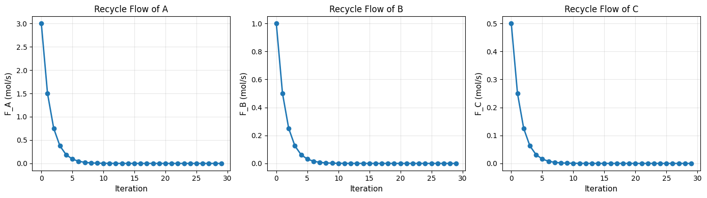
Final converged values:
  F_A = 0.0000 mol/s
  F_B = 0.0000 mol/s
  F_C = 0.0000 mol/s

Part 4: Common Convergence Issues and Solutions

Here’s a reference table for common issues:

issues_table = """
┌─────────────────────────────┬─────────────────────────────────┬─────────────────────────────────────┐
│ Symptom                     │ Likely Cause                    │ Solution                            │
├─────────────────────────────┼─────────────────────────────────┼─────────────────────────────────────┤
│ Oscillating residuals       │ Under-damped iteration          │ Increase damping (0.3-0.5)          │
│                             │                                 │ Use Anderson acceleration           │
├─────────────────────────────┼─────────────────────────────────┼─────────────────────────────────────┤
│ Very slow convergence       │ Poorly conditioned problem      │ Use Anderson acceleration           │
│                             │ Bad initial guess               │ Improve initialization              │
├─────────────────────────────┼─────────────────────────────────┼─────────────────────────────────────┤
│ NaN values                  │ log(0), sqrt(<0), 0/0           │ Add numerical guards                │
│                             │                                 │ Enable jax_debug_nans               │
├─────────────────────────────┼─────────────────────────────────┼─────────────────────────────────────┤
│ Converges to zero flows     │ Poor initialization             │ Use physics-based initial guess     │
│                             │ Unstable steady state           │ Check reaction/separation coupling  │
├─────────────────────────────┼─────────────────────────────────┼─────────────────────────────────────┤
│ Negative concentrations     │ Missing non-negativity guards   │ Add jnp.maximum(x, 0) guards        │
│                             │ Aggressive acceleration         │ Clip accelerated iterates           │
├─────────────────────────────┼─────────────────────────────────┼─────────────────────────────────────┤
│ Flash doesn't converge      │ Two-phase region not exists     │ Check if T, P give valid VLE        │
│                             │ Near bubble/dew point           │ Move away from phase boundary       │
├─────────────────────────────┼─────────────────────────────────┼─────────────────────────────────────┤
│ CSTR temp. doesn't converge │ Strong exotherm + feedback      │ Increase temperature damping        │
│                             │ Multiple steady states          │ Try different initial temperatures  │
└─────────────────────────────┴─────────────────────────────────┴─────────────────────────────────────┘
"""

print("Common Convergence Issues and Solutions")
print(issues_table)

Common Convergence Issues and Solutions

┌─────────────────────────────┬─────────────────────────────────┬─────────────────────────────────────┐
│ Symptom                     │ Likely Cause                    │ Solution                            │
├─────────────────────────────┼─────────────────────────────────┼─────────────────────────────────────┤
│ Oscillating residuals       │ Under-damped iteration          │ Increase damping (0.3-0.5)          │
│                             │                                 │ Use Anderson acceleration           │
├─────────────────────────────┼─────────────────────────────────┼─────────────────────────────────────┤
│ Very slow convergence       │ Poorly conditioned problem      │ Use Anderson acceleration           │
│                             │ Bad initial guess               │ Improve initialization              │
├─────────────────────────────┼─────────────────────────────────┼─────────────────────────────────────┤
│ NaN values                  │ log(0), sqrt(<0), 0/0           │ Add numerical guards                │
│                             │                                 │ Enable jax_debug_nans               │
├─────────────────────────────┼─────────────────────────────────┼─────────────────────────────────────┤
│ Converges to zero flows     │ Poor initialization             │ Use physics-based initial guess     │
│                             │ Unstable steady state           │ Check reaction/separation coupling  │
├─────────────────────────────┼─────────────────────────────────┼─────────────────────────────────────┤
│ Negative concentrations     │ Missing non-negativity guards   │ Add jnp.maximum(x, 0) guards        │
│                             │ Aggressive acceleration         │ Clip accelerated iterates           │
├─────────────────────────────┼─────────────────────────────────┼─────────────────────────────────────┤
│ Flash doesn't converge      │ Two-phase region not exists     │ Check if T, P give valid VLE        │
│                             │ Near bubble/dew point           │ Move away from phase boundary       │
├─────────────────────────────┼─────────────────────────────────┼─────────────────────────────────────┤
│ CSTR temp. doesn't converge │ Strong exotherm + feedback      │ Increase temperature damping        │
│                             │ Multiple steady states          │ Try different initial temperatures  │
└─────────────────────────────┴─────────────────────────────────┴─────────────────────────────────────┘

Part 5: Solver Parameter Tuning

The Flowsheet.solve() method accepts several parameters that can be tuned:

print("Flowsheet.solve() Parameters")
print("=" * 70)
print("""
Parameter         Default   Description
─────────────────────────────────────────────────────────────────────────
tol               1e-8      Convergence tolerance (max residual)
max_iter          100       Maximum iterations before giving up
acceleration      "anderson" Method: "none", "wegstein", or "anderson"
damping           1.0       Step fraction for "none" method (>0; 1.0 = undamped)
anderson_depth    5         History depth for Anderson (higher = more memory)
use_initialization True     Use unit initialize() methods for initial guess
tear_initial      None      Custom initial guess for tear streams
""")

# Demonstrate parameter effects
print("\nEffect of Anderson Depth:")
print("-" * 40)

for depth in [2, 5, 10, 20]:
    result = solve_flowsheet(
        fresh_feed, 
        acceleration="anderson", 
        anderson_depth=depth,
        max_iter=50
    )
    print(f"  depth={depth:2d}: {result['iterations']:3d} iterations, " + 
          f"converged={result['converged']}")

Flowsheet.solve() Parameters
======================================================================

Parameter         Default   Description
─────────────────────────────────────────────────────────────────────────
tol               1e-8      Convergence tolerance (max residual)
max_iter          100       Maximum iterations before giving up
acceleration      "anderson" Method: "none", "wegstein", or "anderson"
damping           1.0       Step fraction for "none" method (>0; 1.0 = undamped)
anderson_depth    5         History depth for Anderson (higher = more memory)
use_initialization True     Use unit initialize() methods for initial guess
tear_initial      None      Custom initial guess for tear streams


Effect of Anderson Depth:
----------------------------------------

  depth= 2:   2 iterations, converged=True

  depth= 5:   2 iterations, converged=True

  depth=10:   2 iterations, converged=True

  depth=20:   2 iterations, converged=True

# Demonstrate tolerance effects
print("\nEffect of Tolerance:")
print("-" * 40)

for tol in [1e-4, 1e-6, 1e-8, 1e-10, 1e-12]:
    result = solve_flowsheet(
        fresh_feed, 
        acceleration="anderson",
        tol=tol,
        max_iter=100
    )
    print(f"  tol={tol:.0e}: {result['iterations']:3d} iterations, " +
          f"residual={result['final_residual']:.2e}")

Effect of Tolerance:
----------------------------------------

  tol=1e-04:   2 iterations, residual=0.00e+00

  tol=1e-06:   2 iterations, residual=0.00e+00

  tol=1e-08:   2 iterations, residual=0.00e+00

  tol=1e-10:   2 iterations, residual=0.00e+00

  tol=1e-12:   2 iterations, residual=0.00e+00

Part 6: Gradient Verification

When gradients through converged solutions look wrong, verify them:

print("Gradient Verification")
print("=" * 50)

# For gradient verification, we need a JIT-compatible solver
# The manual solver above uses Python float() which isn't traceable
# Instead, we'll demonstrate gradient checking on a simpler flowsheet function

def simple_cstr_objective(reactor_volume):
    """Compute product C flow from a single CSTR (no recycle)."""
    cstr_params = CSTRParams(
        V=reactor_volume,
        rate_fn=rate_function,
        stoich=stoichiometry,
        rate_params=rate_params,
        species_order=species_order,
        dH_rxn=jnp.array([-40000.0, -40000.0]),
    )
    cstr = CSTR(cstr_params, thermo=thermo, mode="isothermal")
    
    # Simple inlet
    inlet = make_stream({"A": 10.0, "B": 0.0, "C": 0.0}, T=300.0, P=P_flash)
    outlet, _ = cstr(inlet, T_spec=360.0)
    
    return outlet["F_C"]

# Compute gradient with autodiff
V_base = 10.0  # 10 m³ reactor
grad_autodiff = jax.grad(simple_cstr_objective)(jnp.array(V_base))

# Verify with finite differences
eps = 1e-5
f_plus = simple_cstr_objective(jnp.array(V_base + eps))
f_minus = simple_cstr_objective(jnp.array(V_base - eps))
grad_fd = (f_plus - f_minus) / (2 * eps)

print(f"dF_C/dV at V={V_base} m³:")
print(f"  Autodiff:          {float(grad_autodiff):.6f}")
print(f"  Finite difference: {float(grad_fd):.6f}")
print(f"  Relative error:    {abs(float(grad_autodiff - grad_fd) / float(grad_fd + 1e-10))*100:.4f}%")

print("\nNote: For flowsheets with recycles, use optimistix.implicit_jvp")
print("to get gradients through the converged solution.")

Gradient Verification
==================================================

dF_C/dV at V=10.0 m³:
  Autodiff:          0.000446
  Finite difference: 0.000446
  Relative error:    0.0000%

Note: For flowsheets with recycles, use optimistix.implicit_jvp
to get gradients through the converged solution.

# Using JAX's built-in gradient checker
print("\nUsing jax.test_util.check_grads():")
print("-" * 40)

from jax.test_util import check_grads

# Test gradient correctness on the simple CSTR objective
try:
    check_grads(simple_cstr_objective, (jnp.array(10.0),), order=1, modes=['rev'], eps=1e-4)
    print("Gradient check PASSED")
except AssertionError as e:
    print(f"Gradient check FAILED: {e}")

print("\nTip: Use check_grads() to verify autodiff gradients match finite differences.")

Using jax.test_util.check_grads():
----------------------------------------

Gradient check PASSED

Tip: Use check_grads() to verify autodiff gradients match finite differences.

Summary: Best Practices for Robust Convergence

1. Choose the Right Acceleration Method

• Simple problems: "none" with damping 0.3-0.7

• Moderate problems: "wegstein"

• Difficult problems: "anderson" (usually the best default)

2. Initialize Well

• Use physics-based estimates (reaction conversions, flash splits)

• Start from a nearby solved case if available

• Avoid zero or very small initial flows

3. Add Numerical Guards

• jnp.maximum(x, 1e-10) before log(x) or 1/x

• jnp.clip() for bounded quantities (mole fractions, temperatures)

• Enable jax_debug_nans during development

4. Debug Systematically

• Test units individually before combining

• Visualize residual trajectories

• Use jax.debug.print() inside JIT functions

• Simplify the problem to isolate issues

5. Tune Tolerances Appropriately

• Tighter tolerance = more iterations but more accurate gradients

• For gradient-based optimization, use at least tol=1e-8

• For quick exploration, tol=1e-6 is often sufficient

print("\nKey Takeaways:")
print("─" * 60)
print("""
1. Anderson acceleration is usually the best choice for recycles
2. Good initialization can reduce iterations by 50% or more
3. Numerical guards prevent NaN/Inf from propagating
4. Test units individually when debugging
5. Verify gradients with finite differences when in doubt
""")

Key Takeaways:
────────────────────────────────────────────────────────────

1. Anderson acceleration is usually the best choice for recycles
2. Good initialization can reduce iterations by 50% or more
3. Numerical guards prevent NaN/Inf from propagating
4. Test units individually when debugging
5. Verify gradients with finite differences when in doubt