Updating a Model from Plant Data

28_data_reconciliation.ipynb adjusted measurements to satisfy a model taken as correct. This notebook asks the opposite question: what if the model is the thing that has drifted?

Both are the same optimisation. A variable with a finite \(\sigma\) is a measurement — you may move it, at a cost of \((x-y)^2/\sigma^2\). A variable with \(\sigma = \infty\) is a parameter — move it freely, no cost. That single switch turns reconciliation into estimation, so the interesting question is not how to update a model but when you are entitled to.

The answer matters, because a free parameter can absorb a broken sensor and hand you a confident, wrong number.

What this notebook covers

2. The plant and the model: a pipe that fouls slowly while nobody is looking

3. Forty-five days of operation: monitoring with the model held fixed — the drift shows up in \(\chi^2\)

4. Telling a model fault from an instrument fault (the global test cannot; something else can)

5. Updating the parameter, and checking the update

6. Why you should not leave the parameter free all the time

7. Closing the loop: a gated tracker that applies the discipline automatically

The Summary at the end collects the practical guidance.

1. Setup

import jax
import jax.numpy as jnp

jax.config.update("jax_enable_x64", True)

import numpy as np
import matplotlib.pyplot as plt
import difflow_gas as dg
from difflow_gas import verify
from difflow.reconciliation import (
    blame_concentration,
    global_test,
    measurement_test,
)

# palette: categorical slots 1-2, plus the reserved "critical" status step
BLUE, ORANGE, RED, GREY = "#2a78d6", "#eb6834", "#d03b3b", "#8a8985"
INK, INK_SOFT, GRID = "#0b0b0b", "#52514e", "#eceae6"

def tidy(ax, axis="y"):
    """Recessive axes and grid, so the data carries the emphasis."""
    ax.spines[["top", "right"]].set_visible(False)
    for s in ax.spines.values():
        s.set_color("#d5d4d0")
    ax.tick_params(colors=INK_SOFT, labelsize=8, length=3)
    ax.grid(axis=axis, color=GRID, linewidth=0.8)
    ax.set_axisbelow(True)

RATIOS = {"cs1": 1.2}
P_SLACK_PA = 60.0e5

2. The plant and the model

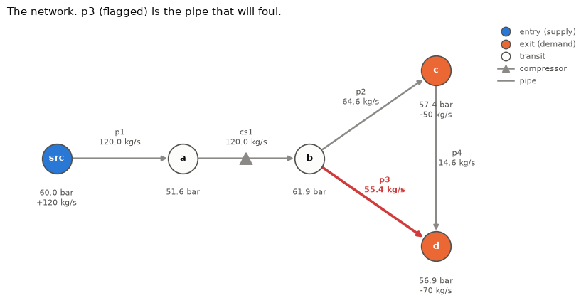
Same five-node network as notebook 28. Pipe p3 is the long leg of the b-c-d loop, and it is the one that will foul: its effective resistance climbs above the design value as deposits build up.

The model always believes p3 is clean. The plant knows better.

def gas_network(eta_p3=1.0):
    """The network, with p3's resistance scaled by eta_p3 (>1 = fouled)."""
    return dg.GasNetwork(
        arcs={
            "p1":  ("src", "a", "pipe"),
            "cs1": ("a",   "b", "compressor"),
            "p2":  ("b",   "c", "pipe"),
            "p3":  ("b",   "d", "pipe"),
            "p4":  ("c",   "d", "pipe"),
        },
        beta={
            aid: dg.weymouth_beta(length_m=L, diameter_m=0.6, roughness_m=1e-4)
                 * (eta_p3 if aid == "p3" else 1.0)
            for aid, L in [("p1", 20e3), ("p2", 40e3), ("p3", 60e3), ("p4", 80e3)]
        },
        supply_kg_s={"src": 120.0, "c": -50.0, "d": -70.0},
    )

def plant_state(eta_p3):
    """The true pressures and flows of a plant whose p3 is fouled by eta_p3."""
    net = gas_network(eta_p3)
    fs, dec = dg.build_network_flowsheet(
        net, root="src", p_slack_pa=P_SLACK_PA, ratios=RATIOS
    )
    streams = fs.solve(tol=1e-12, max_iter=500)
    return (verify.node_pressures_bar(streams, dec),
            verify.arc_flows_kg_s(streams, dec))

model = gas_network(1.0)                     # what the engineers believe
layout = dg.gas_state_layout(model)
sigma = dg.measurement_sigma(layout)         # every variable metered

p0, q0 = plant_state(1.0)
print("clean-plant flows (kg/s):", {k: round(v, 2) for k, v in q0.items()})

clean-plant flows (kg/s): {'p1': 120.0, 'cs1': 120.0, 'p2': 64.61, 'p3': 55.39, 'p4': 14.61}

POS = {"src": (0, 0), "a": (1.15, 0), "b": (2.3, 0),
       "c": (3.45, 0.8), "d": (3.45, -0.8)}

fig, ax = plt.subplots(figsize=(8.5, 4.4))
dg.draw_network(
    model, ax=ax, pos=POS, pressures=p0, flows=q0, highlight=["p3"],
    title="The network. p3 (flagged) is the pipe that will foul.",
)
plt.tight_layout()
plt.show()

3. Forty-five days of operation

Fouling begins on day 12 and grows steadily to 30% excess resistance. Nobody measures it; the only evidence is that the meters stop agreeing with the model.

For contrast we also simulate a second plant where nothing fouls, but the p2 flow meter picks up a \(6\sigma\) bias on day 30. Both faults will push \(\chi^2\) up by a similar amount — which is exactly the difficulty.

DAYS = 45
FOUL_START = 12

eta_true = np.clip(
    1.0 + 0.30 * (np.arange(DAYS) - FOUL_START) / (DAYS - 1 - FOUL_START), 1.0, None
)

# solve the plant once per distinct fouling level, then reuse
levels = {e: plant_state(float(e)) for e in np.unique(np.round(eta_true, 4))}
x_true = {e: layout.pack(p, q, model.supply_kg_s) for e, (p, q) in levels.items()}
print(f"{len(levels)} distinct plant states solved")

33 distinct plant states solved

def simulate(scenario):
    """One day's measurements for each day of the campaign."""
    out = []
    for day in range(DAYS):
        if scenario == "fouling":
            xt = x_true[float(np.round(eta_true[day], 4))]
            gross = None
        else:                                    # clean pipe, bad p2 meter
            xt = x_true[1.0]
            gross = {"q_p2": 6.0} if day >= 30 else None
        out.append(dg.perturb(xt, sigma, jax.random.PRNGKey(1000 + day),
                              layout=layout, gross_errors=gross))
    return out

data_foul = simulate("fouling")
data_sens = simulate("sensor")

# monitor_network reconciles each day against the SAME fixed model and keeps
# the diagnostics. Holding the model and the sigmas still is what makes the
# series readable: every wobble in it comes from the data.
mon_foul = dg.monitor_network(model, data_foul, sigma, layout, ratios=RATIOS)
mon_sens = dg.monitor_network(model, data_sens, sigma, layout, ratios=RATIOS)

chi_foul, chi_sens = mon_foul.statistic, mon_sens.statistic
CRIT = mon_foul.critical

print(f"reject above chi2 = {CRIT:.2f} on {mon_foul.dof} dof")
print(f"last 10 days -- fouling: {chi_foul[-10:].mean():.1f}, "
      f"sensor fault: {chi_sens[-10:].mean():.1f}")

reject above chi2 = 18.31 on 10 dof
last 10 days -- fouling: 37.8, sensor fault: 42.3

fig, axes = plt.subplots(2, 1, figsize=(9.5, 6.0), sharex=True,
                         gridspec_kw={"height_ratios": [1, 2]})

ax = axes[0]
ax.plot(eta_true, color=GREY, linewidth=2)
ax.set_ylabel("true $\\eta$ of p3", fontsize=9, color=INK_SOFT)
ax.set_title("What is actually happening (invisible to the operator)",
             fontsize=10, color=INK, loc="left")
ax.axvline(FOUL_START, color=INK_SOFT, linestyle=(0, (2, 3)), linewidth=1)
ax.text(FOUL_START + 0.7, 1.005, "fouling begins", fontsize=8, color=INK_SOFT)
tidy(ax)

ax = axes[1]
ax.plot(chi_foul, color=BLUE, linewidth=1.8, marker="o", markersize=3.2,
        label="gradual fouling (model drifts)")
ax.plot(chi_sens, color=ORANGE, linewidth=1.8, marker="o", markersize=3.2,
        label="p2 meter bias from day 30 (instrument fault)")
ax.axhline(CRIT, color=RED, linestyle=(0, (4, 3)), linewidth=1.4)
ax.text(DAYS - 0.5, CRIT + 1.5, f"reject above {CRIT:.1f}", fontsize=8,
        color=RED, ha="right")
ax.set_xlabel("day", fontsize=9, color=INK_SOFT)
ax.set_ylabel("global test  $\\chi^2$", fontsize=9, color=INK_SOFT)
ax.set_title("What the operator sees", fontsize=10, color=INK, loc="left")
ax.legend(frameon=False, fontsize=8, loc="upper left", labelcolor=INK_SOFT)
tidy(ax)

plt.tight_layout()
plt.show()

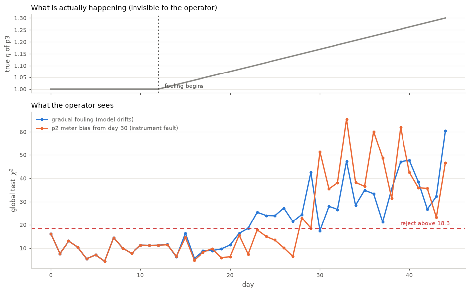
Both faults raise \(\chi^2\) through the threshold, and by the end of the campaign they raise it by a similar amount. The global test says “your data and your model disagree.” It cannot say which of the two is at fault — it never could, because it only measures the size of the disagreement.

4. Telling a model fault from an instrument fault

The measurement test can, but not from any single day. Look at which sensor it blames, day after day.

fig, axes = plt.subplots(1, 2, figsize=(11, 3.6), sharey=True)
order = layout.names

for ax, susp, title, colour in [
    (axes[0], mon_foul.suspects, "Gradual fouling: blame wanders", BLUE),
    (axes[1], mon_sens.suspects, "Meter bias: blame is constant", ORANGE),
]:
    days = [d for d, s in enumerate(susp) if s is not None]
    rows = [order.index(susp[d]) for d in days]
    ax.scatter(days, rows, s=26, color=colour, alpha=0.85)
    none_days = [d for d, s in enumerate(susp) if s is None]
    ax.scatter(none_days, [-1] * len(none_days), s=20, color=GREY, marker="_")
    ax.set_yticks(range(-1, len(order)))
    ax.set_yticklabels(["(nothing flagged)"] + order, fontsize=7.5)
    ax.set_xlabel("day", fontsize=9, color=INK_SOFT)
    ax.set_title(title, fontsize=10, color=INK, loc="left")
    tidy(ax, axis="both")

plt.tight_layout()
plt.show()

# blame_concentration: what fraction of the window blames one single sensor,
# counting the quiet days too -- a campaign that rarely rejects should not
# read as a concentrated fault just because its few rejections agreed.
for tag, mon in [("gradual fouling", mon_foul), ("meter bias", mon_sens)]:
    fraction, culprit = blame_concentration(mon.suspects, window=15)
    print(f"{tag:<16} {fraction:>5.0%} on {culprit}")

print()
print("fouling :", mon_foul.diagnose(window=15))
print("sensor  :", mon_sens.diagnose(window=15))

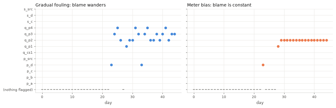
gradual fouling    40% on q_p3
meter bias        100% on q_p2

fouling : model drift: 93% of the last 15 steps reject, blame concentration 40%
sensor  : instrument fault: 100% of the last 15 steps reject, blame concentration 100%, on q_p2

That is the diagnostic. A broken instrument is blamed by name, every day, because the bias sits on one variable and the redundancy points straight at it. A drifting model produces a mismatch the adjustments spread around, so the prime suspect keeps changing and on some days nothing crosses the threshold at all.

diagnose() reads the two together and returns the verdict: persistent rejection with a concentrated suspect is an instrument problem — go and calibrate it; persistent rejection with a diffuse suspect is a model problem, and only then are you entitled to update a parameter. Both thresholds are arguments, so the rule can be tuned to a plant’s own noise; the defaults are half the window rejecting and 60% of it agreeing on one sensor.

5. Updating the parameter

Now, and only now, let \(\eta\) float. One day’s data would give a noisy estimate, so pool a window of days — reconcile_network_multi does that in a single solve, with \(\eta\) appearing once and every day’s equations constraining it.

layout_eta = dg.gas_state_layout(model, efficiency_arcs=["p3"])
sigma_eta = dg.measurement_sigma(layout_eta)      # eta defaults to unmeasured

WINDOW = 10
# embed() re-packs each day's measurements into the layout that carries eta,
# by name -- the added entry is unmeasured, so it is filled with nan.
window = [layout_eta.embed(y, layout) for y in data_foul[-WINDOW:]]

pooled = dg.reconcile_network_multi(
    model, window, sigma_eta, layout_eta, shared=["eta_p3"], ratios=RATIOS
)
eta_hat = pooled.shared["eta_p3"]
eta_sd = pooled.shared_std["eta_p3"]

# for comparison, the same window one day at a time
singles = [
    dg.reconcile_network(model, y, sigma_eta, layout_eta, ratios=RATIOS)
    for y in window
]
per_day = np.array([r.x_named["eta_p3"] for r in singles])
per_day_sd = float(np.mean([r.std["eta_p3"] for r in singles]))

print(f"pooled over the last {WINDOW} days : {eta_hat:.4f} +- {eta_sd:.4f}")
print(f"  averaging the daily estimates  : {per_day.mean():.4f} "
      f"+- {per_day_sd:.4f}  (one day's error bar)")
print(f"  spread across those days       : {per_day.std():.4f}")
print(f"  sqrt({WINDOW}) tighter would be     : "
      f"{per_day_sd / np.sqrt(WINDOW):.4f}")
drift_spread = eta_true[-WINDOW:].std()
print(f"  true eta's own spread in window: {drift_spread:.4f}")
print(f"  one day's error (+) that spread: "
      f"{np.hypot(per_day_sd, drift_spread):.4f}")
print()
print(f"  true mean over the same window : {eta_true[-WINDOW:].mean():.4f}")
print(f"  true value on the final day    : {eta_true[-1]:.4f}")
print()
print(f"degrees of redundancy: {pooled.structure.degree_of_redundancy} "
      f"(vs {singles[0].structure.degree_of_redundancy} x {WINDOW} = "
      f"{singles[0].structure.degree_of_redundancy * WINDOW} "
      f"reconciling separately)")

pooled over the last 10 days : 1.2636 +- 0.0174
  averaging the daily estimates  : 1.2654 +- 0.0551  (one day's error bar)
  spread across those days       : 0.0610
  sqrt(10) tighter would be     : 0.0174
  true eta's own spread in window: 0.0269
  one day's error (+) that spread: 0.0613

  true mean over the same window : 1.2578
  true value on the final day    : 1.3000

degrees of redundancy: 99 (vs 9 x 10 = 90 reconciling separately)

Three things to read here.

The pooled standard error is \(\sqrt{K}\) tighter than a single day’s, and that is not a bookkeeping trick: \(\eta\) appears once in the stacked problem, so each day spends its equations constraining the same unknown instead of ten private copies of it. The degrees of redundancy count it — pooling recovers the nine that ten separate estimations throw away. Averaging the daily point estimates lands in the same place but leaves you holding one day’s error bar for a quantity ten of them informed.

The day-to-day spread (0.061) is the single-day standard error (0.055) plus the drift of the true \(\eta\) across the window (0.027 standard deviation): \(\sqrt{0.055^2 + 0.027^2} = 0.061\). That is the check that the uncertainty is honest — a spread much larger than that would mean the model is missing a source of variation.

And the estimate tracks the window’s average truth, not the final day’s. That lag is unavoidable while the parameter is still moving: any estimate of a drifting quantity is a statement about the recent past, and pooling widens the past it averages over. Choose a window short enough that \(\eta\) is roughly constant across it.

Update the model and re-run the last stretch of the campaign against it.

updated = gas_network(eta_hat)          # the model, corrected

TAIL = 15
chi_before = mon_foul.statistic[-TAIL:]
chi_after = dg.monitor_network(
    updated, data_foul[-TAIL:], sigma, layout, ratios=RATIOS
).statistic

days = np.arange(DAYS - TAIL, DAYS)
fig, ax = plt.subplots(figsize=(9, 3.8))
ax.plot(days, chi_before, color=BLUE, linewidth=1.8, marker="o", markersize=3.5,
        label="original model")
ax.plot(days, chi_after, color=ORANGE, linewidth=1.8, marker="o", markersize=3.5,
        label=f"model updated to $\\eta$ = {eta_hat:.3f}")
ax.axhline(CRIT, color=RED, linestyle=(0, (4, 3)), linewidth=1.4)
ax.text(days[-1], CRIT + 1.2, f"reject above {CRIT:.1f}", fontsize=8, color=RED,
        ha="right")
ax.set_xlabel("day", fontsize=9, color=INK_SOFT)
ax.set_ylabel("global test  $\\chi^2$", fontsize=9, color=INK_SOFT)
ax.set_title("The same measurements, before and after the model update",
             fontsize=10, color=INK, loc="left")
ax.legend(frameon=False, fontsize=8, loc="upper right", labelcolor=INK_SOFT)
tidy(ax)
plt.tight_layout()
plt.show()

print(f"mean chi2  before {chi_before.mean():6.2f}   after {chi_after.mean():6.2f}"
      f"   (expected ~{mon_foul.dof} on {mon_foul.dof} dof if the model is right)")
print()
print(f"days still over {CRIT:.2f} after the update (window was days "
      f"{DAYS - WINDOW}-{DAYS - 1}):")
for d, c in zip(days, chi_after):
    if c > CRIT:
        print(f"  day {d}: chi2 {c:5.1f}   true eta {eta_true[d]:.3f}   "
              f"(model assumes {eta_hat:.3f})")
last5 = np.asarray(chi_after[-5:])
print(f"last 5 days (true eta {eta_true[-5]:.3f}-{eta_true[-1]:.3f}): "
      f"chi2 {last5.min():.1f}-{last5.max():.1f}")

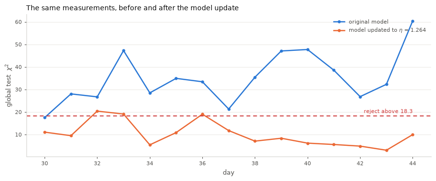
mean chi2  before  35.04   after  10.12   (expected ~10 on 10 dof if the model is right)

days still over 18.31 after the update (window was days 35-44):
  day 32: chi2  20.4   true eta 1.188   (model assumes 1.264)
  day 33: chi2  19.1   true eta 1.197   (model assumes 1.264)
  day 36: chi2  19.0   true eta 1.225   (model assumes 1.264)
last 5 days (true eta 1.262-1.300): chi2 3.0-9.9

The same data that rejected the old model is unremarkable against the updated one. Nothing about the measurements changed — only what we now believe about the pipe.

Three days (32, 33 and 36) still brush the threshold. All three sit early in the 15-day tail, where the pipe really was cleaner (true \(\eta\) 1.19–1.23) than the 1.264 the update assumes, and two of them fall before the 10-day window \(\eta\) was estimated from. It is the caveat below, seen from close up. The final days, where the pipe has become dirtier than the window average, are still comfortably inside the limit (\(\chi^2\) 3.0–9.9); the lag would show up there as the fouling continues.

One caveat worth being explicit about: the updated model describes the plant as it is now. Re-run it against day 15’s data and it will reject, correctly, because the pipe really was cleaner then. A parameter update is a statement about the present, not a retroactive correction, and fouling that keeps progressing will need updating again.

6. Why not just leave the parameter free?

If a free \(\eta\) fixes a drifting model, why fix it at all? Because a free parameter absorbs whatever is wrong — including a lying sensor.

Feed the instrument-fault data to a reconciliation with \(\eta\) free, and watch it manufacture a fouling estimate out of a bad meter.

y_bad = data_sens[-1]                          # p2 meter biased, pipe is clean
y_bad_eta = layout_eta.embed(y_bad, layout)

fixed = dg.reconcile_network(model, y_bad, sigma, layout, ratios=RATIOS)
free = dg.reconcile_network(model, y_bad_eta, sigma_eta, layout_eta, ratios=RATIOS)

print(f"{'':22} {'chi2':>8} {'verdict':>10} {'suspect':>9} {'eta estimate':>16}")
print("-" * 70)
for tag, res, eta in [("parameter fixed", fixed, None),
                      ("parameter free", free,
                       (free.x_named["eta_p3"], free.std["eta_p3"]))]:
    g, m = global_test(res), measurement_test(res)
    print(f"{tag:22} {g.statistic:8.2f} {'REJECT' if g.detected else 'accept':>10} "
          f"{str(m.suspect):>9} "
          f"{('fixed at 1.000' if eta is None else f'{eta[0]:.3f} +- {eta[1]:.3f}'):>16}")

print(f"\nthe pipe is genuinely clean (eta = 1.000)")

                           chi2    verdict   suspect     eta estimate
----------------------------------------------------------------------
parameter fixed           46.67     REJECT      q_p2   fixed at 1.000
parameter free            25.25     REJECT      q_p2   1.221 +- 0.053

the pipe is genuinely clean (eta = 1.000)

With \(\eta\) free the statistic falls, because the parameter has soaked up part of the bias — and the fouling estimate it reports is not 1.0. A single meter fault has been converted into a confident statement about a pipe nobody inspected.

That is the whole argument for the two-clock discipline below. In the routine loop the model has no freedom, so the \(\chi^2\) test is a genuine instrument-health monitor. Give the model freedom and the monitor goes soft: the statistic falls by half while a fouling factor of 1.22 \(\pm\) 0.05 appears on a clean pipe. Here the bias is large enough that the test still rejects and still names q_p2. A smaller bias, or a parameter placed to absorb it more completely, would slip under the threshold with the invented fouling intact.

7. Closing the loop

Sections 3 to 5 describe a discipline a person applies: watch the monitor, read the verdict, decide you are entitled to re-estimate, pool a window, rebuild the model. A digital twin — a model kept current so that what you optimise and price against is the plant as it is — has nobody to apply it. Automating it naively breaks it in two places.

The verdict has to gate the update, not advise it. Section 6 is what happens otherwise: the free parameter absorbs the meter bias, reports fouling on a clean pipe, and \(\chi^2\) falls while it does. Nothing about a slower update prevents that — it would just arrive at the same wrong number more gradually.

The update needs a memory. The pooled estimate of section 5 is a rectangular filter: hard edges, a ten-day-old day weighted like today, rebuilt from scratch each time. Re-run it on a schedule and the estimate lurches as days fall off the back.

track_parameters is those two fixes. Each day it reconciles with \(\eta\) frozen at the current estimate (clock one, so the tests still mean something), reads the verdict, and only where the verdict is model drift does it estimate \(\eta\) from that day and fold the result into a random walk (clock two).

from difflow.reconciliation import (
    TrackerState, drift_std_from_time_constant, track_parameters,
)

# One residual function serves both clocks. eta_p3 arrives through `params`
# rather than baked into the network, because GasNetwork validates its
# arguments with Python comparisons and so cannot be built under a trace.
def gas_residuals(x, params):
    return dg.residuals.network_residuals(
        x, model, layout, ratios=RATIOS,
        efficiencies={"p3": params["eta_p3"]},
    )

# "the pipe might foul by 10% in a month" -- the question an engineer can
# actually answer -- converted into the random-walk rate the filter wants.
DRIFT = drift_std_from_time_constant(0.10, 30.0)

# The diagnose() rule, tuned to this network. At the defaults (window 15,
# 60% concentration) a couple of days of the meter-bias campaign read as
# diffuse and slip through the gate; a longer window fixes it. Tuning the
# rule is the right response to that -- widening `allow` is not.
GATE = dict(window=21, concentration_threshold=0.4)

def track(data, **kw):
    run = track_parameters(
        gas_residuals, data, sigma,
        state=TrackerState.initial(["eta_p3"], [1.0], std=[0.02]),
        drift_std=DRIFT, names=layout.names,
        unmeasured_scale=layout.default_scale, **GATE, **kw,
    )
    jax.clear_caches()        # each day traces a fresh closure
    return run

tracked = track(data_foul)

first = next(s.index for s in tracked.steps if s.updated)
print(f"drift_std        {float(DRIFT):.4f} per day")
print(f"first update     day {first}   (fouling began on day {FOUL_START})")
print(f"final estimate   {tracked.of('eta_p3')[-1]:.3f} "
      f"+- {tracked.std_of('eta_p3')[-1]:.3f}   (true {eta_true[-1]:.3f})")
print(f"updates          {tracked.n_updates} of {len(tracked)} days")

drift_std        0.0183 per day
first update     day 33   (fouling began on day 12)
final estimate   1.257 +- 0.039   (true 1.300)
updates          10 of 45 days

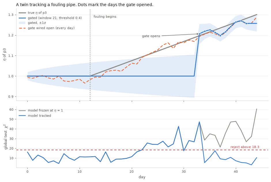
The loop spends most of the campaign doing nothing, which is the design. While the verdict is consistent the gate stays shut and \(\eta\) does not move — but the time update still runs, so its error bar widens day by day at the drift rate. A held parameter is not a known parameter, and the twin says so.

Then the evidence accumulates, the verdict flips, and the gate opens.

For contrast, run the same filter with the gate wired open — re-estimating every day regardless of the verdict.

from difflow.reconciliation import (
    MONITOR_CONSISTENT, MONITOR_INSTRUMENT_FAULT, MONITOR_MODEL_DRIFT,
    MONITOR_UNDIAGNOSED,
)

EVERY_DAY = [MONITOR_CONSISTENT, MONITOR_INSTRUMENT_FAULT,
             MONITOR_MODEL_DRIFT, MONITOR_UNDIAGNOSED]
ungated = track(data_foul, allow=EVERY_DAY)

days = np.arange(DAYS)
eta_g, eta_u = tracked.of("eta_p3"), ungated.of("eta_p3")
sd_g = tracked.std_of("eta_p3")
marks = [s.index for s in tracked.steps if s.updated]

fig, axes = plt.subplots(2, 1, figsize=(9.5, 6.4), sharex=True,
                         gridspec_kw={"height_ratios": [3, 2]})

ax = axes[0]
ax.plot(days, eta_true, color=GREY, linewidth=2.4, label="true $\\eta$ of p3")
ax.fill_between(days, eta_g - sd_g, eta_g + sd_g, color=BLUE, alpha=0.13,
                linewidth=0, label="gated, $\\pm 1\\sigma$")
ax.plot(days, eta_u, color=ORANGE, linewidth=1.8, linestyle=(0, (4, 2)),
        label="gate wired open (every day)")
ax.plot(days, eta_g, color=BLUE, linewidth=2.0, label="gated (window 21, threshold 0.4)")
ax.plot(marks, eta_g[marks], linestyle="none", marker="o", markersize=4.5,
        color=BLUE, markeredgecolor="white", markeredgewidth=0.8)
ax.axvline(FOUL_START, color=INK_SOFT, linestyle=(0, (2, 3)), linewidth=1)
ax.text(FOUL_START + 0.7, 1.285, "fouling begins", fontsize=8, color=INK_SOFT)
ax.annotate("gate opens", xy=(first, eta_g[first]), xytext=(first - 11, 1.19),
            fontsize=8, color=INK_SOFT,
            arrowprops=dict(arrowstyle="->", color=INK_SOFT, linewidth=0.9))
ax.set_ylim(0.88, 1.33)          # the held band is wide on purpose
ax.set_ylabel("$\\eta$ of p3", fontsize=9, color=INK_SOFT)
ax.set_title("A twin tracking a fouling pipe. Dots mark the days the gate opened.",
             fontsize=10, color=INK, loc="left")
h, l = ax.get_legend_handles_labels()
order = [l.index(k) for k in ["true $\\eta$ of p3", "gated (window 21, threshold 0.4)",
                              "gated, $\\pm 1\\sigma$",
                              "gate wired open (every day)"]]
ax.legend([h[k] for k in order], [l[k] for k in order], frameon=False,
          fontsize=8, loc="upper left", labelcolor=INK_SOFT)
tidy(ax)

ax = axes[1]
ax.plot(days, mon_foul.statistic, color=GREY, linewidth=1.7,
        label="model frozen at $\\eta$ = 1")
ax.plot(days, tracked.monitor.statistic, color=BLUE, linewidth=1.7,
        label="model tracked")
ax.axhline(CRIT, color=RED, linestyle=(0, (4, 3)), linewidth=1.4)
ax.text(DAYS - 0.5, CRIT + 2.0, f"reject above {CRIT:.1f}", fontsize=8,
        color=RED, ha="right")
ax.set_xlabel("day", fontsize=9, color=INK_SOFT)
ax.set_ylabel("global test  $\\chi^2$", fontsize=9, color=INK_SOFT)
ax.legend(frameon=False, fontsize=8, loc="upper left", labelcolor=INK_SOFT)
tidy(ax)

plt.tight_layout()
plt.show()

tail = slice(-10, None)
print(f"{'':34} {'final eta':>10} {'mean |err| last 10 d':>22} {'updates':>9}")
print("-" * 78)
for tag, e, r in [("gated (window 21, threshold 0.4)", eta_g, tracked),
                  ("gate wired open", eta_u, ungated)]:
    print(f"{tag:34} {e[-1]:10.3f} "
          f"{np.abs(e[tail] - eta_true[tail]).mean():22.4f} {r.n_updates:9d}")

                                    final eta   mean |err| last 10 d   updates
------------------------------------------------------------------------------
gated (window 21, threshold 0.4)        1.257                 0.0200        10
gate wired open                         1.288                 0.0178        45

Two things to read.

The loop closes. The lower panel is the same data scored against a model that moves. Frozen at \(\eta = 1\) it rejects for the whole back half of the campaign; tracked, it drops back under the threshold after each update and stays there. That is the test doing its job again — and a \(\chi^2\) that failed to come back down would be the signal that no value of \(\eta\) fits and the mismatch is structural.

The gate costs accuracy, and that is the trade. Opening it every day tracks the drift slightly better, because it never waits for evidence. The gated loop lags: fouling starts on day 12 and runs for three weeks before the gate opens on day 33. From about day 22 the monitor is already rejecting, so for the last stretch of that the twin holds a model it has reason to doubt — and says so through a widening error bar rather than by guessing.

Whether that lag is worth paying is decided by the other campaign.

sens_gated = track(data_sens)
sens_open = track(data_sens, allow=EVERY_DAY)

print("the p2 meter is biased from day 30; the pipe is genuinely clean "
      "(eta = 1.000)\n")
print(f"{'':34} {'fouling campaign':>18} {'meter-bias campaign':>21}")
print("-" * 78)
for tag, a, b in [("gated (window 21, threshold 0.4)", tracked, sens_gated),
                  ("gate wired open", ungated, sens_open)]:
    print(f"{tag:34} {a.of('eta_p3')[-1]:18.3f} "
          f"{b.of('eta_p3')[-1]:21.3f}")
print(f"{'true value':34} {eta_true[-1]:18.3f} {1.0:21.3f}")
print()

from collections import Counter
print("verdicts on the meter-bias campaign:",
      dict(Counter(s.diagnosis.verdict for s in sens_gated.steps)))
print(f"updates: {sens_gated.n_updates} gated, {sens_open.n_updates} wired open")

the p2 meter is biased from day 30; the pipe is genuinely clean (eta = 1.000)

                                     fouling campaign   meter-bias campaign
------------------------------------------------------------------------------
gated (window 21, threshold 0.4)                1.257                 1.000
gate wired open                                 1.288                 1.165
true value                                      1.300                 1.000

verdicts on the meter-bias campaign: {'consistent': 38, 'instrument fault': 7}
updates: 0 gated, 45 wired open

There is the answer. Read the columns together:

	fouling campaign	meter-bias campaign
gated (window 21, threshold 0.4)	1.257 (true 1.300) — lags	1.000 — correct, never moved
wired open	1.288 (true 1.300) — tracks	1.165 — fouling invented

Opening the gate buys about 0.03 in \(\eta\) on the campaign where the model really was wrong, and costs a confident 16% fouling claim on a pipe that was clean. The gated loop never updates on the meter-bias campaign at all: every day is either consistent or instrument fault, and neither entitles the model to move. What it reports instead is a widening error bar on \(\eta\) and a named suspect to go and calibrate — which is the correct output, because the pipe is fine and the meter is not.

# The same gate at the LIBRARY defaults (window=15, concentration_threshold=0.6),
# not the tuned GATE used above -- on the meter-bias campaign, where any update
# is a mistake.
sens_defaults = track_parameters(
    gas_residuals, data_sens, sigma,
    state=TrackerState.initial(["eta_p3"], [1.0], std=[0.02]),
    drift_std=DRIFT, names=layout.names,
    unmeasured_scale=layout.default_scale,
)
jax.clear_caches()

upd = [s for s in sens_defaults.steps if s.updated]
print("gate at the library defaults, meter-bias campaign (true eta = 1.000)")
print(f"  gated updates : {sens_defaults.n_updates}")
for s in upd:
    print(f"    day {s.index}: verdict {s.diagnosis.verdict!r}, "
          f"eta -> {sens_defaults.of('eta_p3')[s.index]:.3f}")
print(f"  final eta     : {sens_defaults.of('eta_p3')[-1]:.3f}")

gate at the library defaults, meter-bias campaign (true eta = 1.000)
  gated updates : 2
    day 35: verdict 'model drift', eta -> 1.143
    day 36: verdict 'model drift', eta -> 1.131
  final eta     : 1.131

One caveat, and it is why window and concentration_threshold are arguments above rather than fixed. The gate is a statistical rule, not a guarantee. At the library defaults (window=15, concentration_threshold=0.6 — not the tuned 21 / 0.4 used earlier) on this small network two days early in the bias (35 and 36) read as diffuse, slip through as model drift, and drag \(\eta\) to 1.131 before the rule settles — the run above this paragraph. The fix is to tune the rule to the plant’s own noise — lengthen the window, lower the concentration threshold — and track_parameters forwards both to diagnose. The fix is not to widen allow, which removes the rule rather than sharpening it.

What this still does not fix. The filter corrects a parameter, not the model’s form. If the network were wrong in shape — a missing leg, the wrong pipe law — no value of \(\eta\) would fit, \(\chi^2\) would stay above the line after every update, and the twin’s gradients would be wrong even on days its values happened to match. That is fatal for a differentiable flowsheet, where everything downstream is a derivative. difflow.planning.modifiers corrects values and gradients together and is the right tool there; a faster filter is not.

Summary

	Data reconciliation	Parameter estimation
What moves	the measurements	the model coefficients
In code	finite sigma	sigma = inf
Assumes	model right, sensors wrong	sensors right, model wrong
Costs	nothing	one degree of redundancy each

They are one optimisation, separated only by which weights you set to zero. What separates them in practice is the discipline about when each is allowed to run.

Two clocks

• Routine (hourly, daily): parameters fixed. monitor_network runs this one. The \(\chi^2\) test is then a real instrument-health monitor, because the model cannot flex to hide a fault, and diagnose() reads the series for you.

• Campaign (weekly, monthly): re-estimate parameters. reconcile_network_multi pools the window. Trigger it on persistent rejection with a diffuse suspect — the signature of a model fault, section 4 — never on a single bad day, and never on a concentrated suspect, which means go calibrate a meter instead.

Both clocks, run for you. track_parameters (section 7) is the pair written as an update law, for a twin where nobody is there to apply the discipline by hand. The verdict gates the re-estimation instead of advising it, and what gets through is filtered onto a random walk whose rate you choose — so the parameter moves at a pace you set rather than at the pace one day’s noise suggests. The cost is a detection lag; the thing it buys is that a biased meter never becomes a statement about a pipe.

Reading the two tests together

\(\chi^2\)	suspect	reading
accept	—	healthy
reject once	any	noise, or a transient; wait
reject persistently	same name every day	instrument fault — calibrate it
reject persistently	wanders, often none	model drift — estimate the parameter

What the differentiability bought here: the parameter update is not a separate fitting code path. It is the same reconcile call with one sigma set to infinity, and the standard error on \(\eta\) comes from the same covariance matrix as every reconciled flow. Pooling a window does not change that either — it stacks the same KKT system over ten days with \(\eta\) shared, which is why its error bar shrinks by \(\sqrt{10}\) and its degrees of redundancy go up rather than down.