
Surrogate Models for Unit Operations: Pump Example#
This notebook demonstrates how to create and use neural network surrogate models for unit operations within the difflow framework.
Topics covered:
Physics-based pump model (ground truth)
Static surrogate pump using neural networks
Training the static surrogate
Dynamic surrogate pump with startup transients
Training the dynamic surrogate
Using surrogates in flowsheets
Gradient-based optimization through surrogates
import jax
import jax.numpy as jnp
from jax import random, grad, vmap, jit
import matplotlib.pyplot as plt

# Configure JAX
jax.config.update("jax_enable_x64", True)

# Import difflow
from difflow.streams import make_stream, get_flows, total_flow
from difflow.dynamic import (
    DynamicUnitBase,
    StateSpec,
    StateVar,
    StateVector,
    integrate_unit,
    integrate,
    pressure_state,
)

print(f"JAX version: {jax.__version__}")
WARNING:2026-01-10 19:57:33,192:jax._src.xla_bridge:852: An NVIDIA GPU may be present on this machine, but a CUDA-enabled jaxlib is not installed. Falling back to cpu.
JAX version: 0.8.2
1. Physics-Based Pump Model (Ground Truth)#
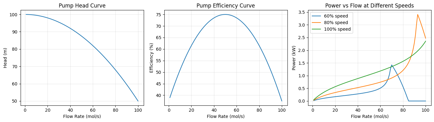
First, let’s create a physics-based pump model that we’ll use to generate training data.
A centrifugal pump can be characterized by:
Head-flow curve: \(H = H_0 - a Q^2\) (parabolic)
Efficiency curve: \(\eta = \eta_{max} \cdot (1 - b(Q - Q_{opt})^2)\)
Power: \(P = \rho g Q H / \eta\)
Pressure rise: \(\Delta P = \rho g H\)
For simplicity, we’ll work with molar flow rates and assume constant density.
class PhysicsPump:
    """Physics-based centrifugal pump model.

    This serves as our 'ground truth' for generating training data.

    The pump curves are defined in terms of molar flow rate (mol/s) for
    direct compatibility with difflow streams. For a real pump, you would
    convert between molar and volumetric flow using fluid density and MW.
    """

    def __init__(
        self,
        H0: float = 100.0,      # Shutoff head (m) - increased for positive head at high flows
        a: float = 0.005,       # Head curve coefficient (m/(mol/s)^2) - reduced slope
        eta_max: float = 0.75,  # Maximum efficiency
        F_opt: float = 50.0,    # Optimal molar flow rate (mol/s)
        b: float = 0.0002,      # Efficiency curve width ((mol/s)^-2) - wider curve
        rho: float = 1000.0,    # Fluid density (kg/m³)
        MW: float = 0.018,      # Molecular weight (kg/mol) - water
    ):
        self.H0 = H0
        self.a = a
        self.eta_max = eta_max
        self.F_opt = F_opt
        self.b = b
        self.rho = rho
        self.MW = MW
        self.g = 9.81  # m/s²

    def head(self, F: jnp.ndarray) -> jnp.ndarray:
        """Pump head (m) as function of molar flow rate (mol/s)."""
        return self.H0 - self.a * F**2

    def efficiency(self, F: jnp.ndarray) -> jnp.ndarray:
        """Pump efficiency as function of molar flow rate (mol/s)."""
        eta = self.eta_max * (1 - self.b * (F - self.F_opt)**2)
        return jnp.clip(eta, 0.1, self.eta_max)  # Minimum efficiency

    def __call__(self, inlet, speed_fraction: float = 1.0):
        """Process inlet stream through pump.

        Args:
            inlet: Input stream dict with F_*, T, P
            speed_fraction: Pump speed as fraction of rated (0-1)

        Returns:
            (outlet_stream, info_dict)
        """
        # Get molar flow rate
        F_total = total_flow(inlet)

        # Apply affinity laws for speed variation
        # Q ∝ N, H ∝ N², P ∝ N³
        F_eff = F_total / speed_fraction  # Equivalent flow at rated speed

        # Calculate head and efficiency at rated speed
        H_rated = self.head(F_eff)
        eta = self.efficiency(F_eff)

        # Apply affinity laws
        H = H_rated * speed_fraction**2

        # Ensure non-negative head (pump cannot create suction)
        H = jnp.maximum(H, 0.0)

        # Pressure rise: dP = rho * g * H
        dP = self.rho * self.g * H
        P_out = inlet['P'] + dP

        # Power consumption: volumetric flow * dP / efficiency
        # Convert molar flow to volumetric: Q_vol = F * MW / rho
        Q_vol = F_total * self.MW / self.rho  # m³/s
        power = Q_vol * dP / (eta + 1e-10)  # W

        # Temperature rise from inefficiency (simplified)
        # Q_waste = power * (1 - eta)
        # dT = Q_waste / (F_total * Cp)
        Cp = 75.0  # J/mol/K (water)
        dT = power * (1 - eta) / (F_total * Cp + 1e-10)
        T_out = inlet['T'] + dT

        # Create outlet stream (same composition, new T and P)
        outlet_flows = get_flows(inlet)
        outlet = make_stream(outlet_flows, T_out, P_out)

        info = {
            'head': H,
            'efficiency': eta,
            'power': power,
            'dP': dP,
            'dT': dT,
        }

        return outlet, info


# Create physics pump
physics_pump = PhysicsPump()

# Test it
inlet = make_stream({'water': 50.0}, T=300.0, P=101325.0)
outlet, info = physics_pump(inlet, speed_fraction=1.0)

print("Physics Pump Test:")
print(f"  Inlet:  F={total_flow(inlet):.1f} mol/s, T={inlet['T']:.1f} K, P={inlet['P']/1000:.1f} kPa")
print(f"  Outlet: F={total_flow(outlet):.1f} mol/s, T={outlet['T']:.2f} K, P={outlet['P']/1000:.1f} kPa")
print(f"  Head: {info['head']:.2f} m")
print(f"  Efficiency: {info['efficiency']*100:.1f}%")
print(f"  Power: {info['power']:.1f} W")
Physics Pump Test:
  Inlet:  F=50.0 mol/s, T=300.0 K, P=101.3 kPa
  Outlet: F=50.0 mol/s, T=300.07 K, P=959.7 kPa
  Head: 87.50 m
  Efficiency: 75.0%
  Power: 1030.0 W
Visualize Pump Curves#
# Generate pump curves
F_range = jnp.linspace(1, 100, 100)

fig, axes = plt.subplots(1, 3, figsize=(14, 4))

# Head curve
H_curve = vmap(physics_pump.head)(F_range)
axes[0].plot(F_range, H_curve)
axes[0].set_xlabel('Flow Rate (mol/s)')
axes[0].set_ylabel('Head (m)')
axes[0].set_title('Pump Head Curve')
axes[0].grid(True, alpha=0.3)

# Efficiency curve
eta_curve = vmap(physics_pump.efficiency)(F_range)
axes[1].plot(F_range, eta_curve * 100)
axes[1].set_xlabel('Flow Rate (mol/s)')
axes[1].set_ylabel('Efficiency (%)')
axes[1].set_title('Pump Efficiency Curve')
axes[1].grid(True, alpha=0.3)

# Power curve at different speeds
for speed in [0.6, 0.8, 1.0]:
    powers = []
    for F in F_range:
        inlet = make_stream({'water': float(F)}, T=300.0, P=101325.0)
        _, info = physics_pump(inlet, speed_fraction=speed)
        powers.append(info['power'])
    axes[2].plot(F_range, jnp.array(powers) / 1000, label=f'{speed*100:.0f}% speed')

axes[2].set_xlabel('Flow Rate (mol/s)')
axes[2].set_ylabel('Power (kW)')
axes[2].set_title('Power vs Flow at Different Speeds')
axes[2].legend()
axes[2].grid(True, alpha=0.3)

plt.tight_layout()
plt.show()
2. Static Surrogate Pump Model#
Now let’s create a neural network surrogate that learns the pump behavior.
The surrogate will:
Input: Flow rate, inlet temperature, inlet pressure, pump speed
Output: Pressure rise, temperature rise, power consumption
def init_mlp(key, layer_sizes):
    """Initialize MLP parameters.

    Args:
        key: JAX random key
        layer_sizes: List of layer sizes [input, hidden1, ..., output]

    Returns:
        List of (weights, biases) tuples
    """
    params = []
    for i in range(len(layer_sizes) - 1):
        key, subkey = random.split(key)
        in_size, out_size = layer_sizes[i], layer_sizes[i + 1]
        # Xavier initialization
        scale = jnp.sqrt(2.0 / (in_size + out_size))
        w = random.normal(subkey, (out_size, in_size)) * scale
        b = jnp.zeros(out_size)
        params.append((w, b))
    return params


def mlp_forward(params, x):
    """Forward pass through MLP.

    Args:
        params: List of (weights, biases)
        x: Input array

    Returns:
        Output array
    """
    for i, (w, b) in enumerate(params):
        x = w @ x + b
        # ReLU activation except for last layer
        if i < len(params) - 1:
            x = jax.nn.relu(x)
    return x


class SurrogatePump:
    """Neural network surrogate for pump model.

    Input features (normalized):
        - Flow rate (mol/s)
        - Inlet temperature (K)
        - Inlet pressure (Pa)
        - Pump speed fraction

    Output predictions:
        - Pressure rise (Pa)
        - Temperature rise (K)
        - Power consumption (W)
    """

    def __init__(self, nn_params, input_scale, output_scale):
        """Initialize surrogate pump.

        Args:
            nn_params: Neural network parameters
            input_scale: (mean, std) for input normalization
            output_scale: (mean, std) for output denormalization
        """
        self.nn_params = nn_params
        self.input_mean, self.input_std = input_scale
        self.output_mean, self.output_std = output_scale

    def predict_raw(self, features):
        """Raw NN prediction (normalized in/out)."""
        x_norm = (features - self.input_mean) / (self.input_std + 1e-8)
        y_norm = mlp_forward(self.nn_params, x_norm)
        return y_norm * self.output_std + self.output_mean

    def __call__(self, inlet, speed_fraction: float = 1.0):
        """Process inlet stream through surrogate pump.

        Follows the same interface as PhysicsPump.
        """
        # Extract features
        F_total = total_flow(inlet)
        features = jnp.array([
            F_total,
            inlet['T'],
            inlet['P'],
            speed_fraction,
        ])

        # Neural network prediction
        outputs = self.predict_raw(features)
        dP, dT, power = outputs[0], outputs[1], outputs[2]

        # Ensure physical constraints
        dP = jnp.maximum(dP, 0.0)  # Pressure can only increase
        power = jnp.maximum(power, 0.0)  # Power is positive

        # Create outlet stream
        outlet_flows = get_flows(inlet)
        T_out = inlet['T'] + dT
        P_out = inlet['P'] + dP
        outlet = make_stream(outlet_flows, T_out, P_out)

        info = {
            'dP': dP,
            'dT': dT,
            'power': power,
        }

        return outlet, info


# Initialize network architecture
key = random.PRNGKey(42)
layer_sizes = [4, 32, 32, 3]  # 4 inputs, 2 hidden layers, 3 outputs
nn_params = init_mlp(key, layer_sizes)

print(f"Network architecture: {layer_sizes}")
print(f"Total parameters: {sum(w.size + b.size for w, b in nn_params)}")
Network architecture: [4, 32, 32, 3]
Total parameters: 1315
3. Training the Static Surrogate#
Generate training data from the physics model and train the neural network.
def generate_training_data(pump, n_samples, key):
    """Generate training data from physics pump.

    Returns:
        X: Input features (n_samples, 4)
        Y: Output targets (n_samples, 3)
    """
    keys = random.split(key, 4)

    # Sample operating conditions
    flows = random.uniform(keys[0], (n_samples,), minval=5.0, maxval=100.0)
    temps = random.uniform(keys[1], (n_samples,), minval=280.0, maxval=350.0)
    pressures = random.uniform(keys[2], (n_samples,), minval=50000.0, maxval=200000.0)
    speeds = random.uniform(keys[3], (n_samples,), minval=0.5, maxval=1.0)

    X = []
    Y = []

    for i in range(n_samples):
        inlet = make_stream({'water': float(flows[i])}, T=float(temps[i]), P=float(pressures[i]))
        outlet, info = pump(inlet, speed_fraction=float(speeds[i]))

        x = [flows[i], temps[i], pressures[i], speeds[i]]
        y = [info['dP'], info['dT'], info['power']]

        X.append(x)
        Y.append(y)

    return jnp.array(X), jnp.array(Y)


# Generate data
n_train = 1000
n_test = 200

key, subkey = random.split(key)
X_train, Y_train = generate_training_data(physics_pump, n_train, subkey)

key, subkey = random.split(key)
X_test, Y_test = generate_training_data(physics_pump, n_test, subkey)

# Compute normalization statistics
input_mean = jnp.mean(X_train, axis=0)
input_std = jnp.std(X_train, axis=0)
output_mean = jnp.mean(Y_train, axis=0)
output_std = jnp.std(Y_train, axis=0)

print(f"Training samples: {n_train}")
print(f"Test samples: {n_test}")
print(f"\nInput statistics:")
print(f"  Flow:     mean={input_mean[0]:.1f}, std={input_std[0]:.1f}")
print(f"  Temp:     mean={input_mean[1]:.1f}, std={input_std[1]:.1f}")
print(f"  Pressure: mean={input_mean[2]:.0f}, std={input_std[2]:.0f}")
print(f"  Speed:    mean={input_mean[3]:.2f}, std={input_std[3]:.2f}")
print(f"\nOutput statistics:")
print(f"  dP:    mean={output_mean[0]:.0f} Pa, std={output_std[0]:.0f}")
print(f"  dT:    mean={output_mean[1]:.4f} K, std={output_std[1]:.4f}")
print(f"  Power: mean={output_mean[2]:.0f} W, std={output_std[2]:.0f}")
Training samples: 1000
Test samples: 200

Input statistics:
  Flow:     mean=52.9, std=27.4
  Temp:     mean=315.3, std=19.8
  Pressure: mean=126086, std=42913
  Speed:    mean=0.74, std=0.14

Output statistics:
  dP:    mean=394827 Pa, std=249729
  dT:    mean=0.0876 K, std=0.0734
  Power: mean=693 W, std=608
def loss_fn(params, X_batch, Y_batch, input_scale, output_scale):
    """Mean squared error loss."""
    input_mean, input_std = input_scale
    output_mean, output_std = output_scale

    def predict(x):
        x_norm = (x - input_mean) / (input_std + 1e-8)
        y_norm = mlp_forward(params, x_norm)
        return y_norm * output_std + output_mean

    Y_pred = vmap(predict)(X_batch)

    # Normalize loss by output scale for balanced gradients
    errors = (Y_pred - Y_batch) / (output_std + 1e-8)
    return jnp.mean(errors**2)


def update_step(params, X_batch, Y_batch, learning_rate, input_scale, output_scale):
    """Single SGD update step."""
    loss, grads = jax.value_and_grad(loss_fn)(params, X_batch, Y_batch, input_scale, output_scale)

    # Update parameters
    new_params = []
    for (w, b), (dw, db) in zip(params, grads):
        new_params.append((
            w - learning_rate * dw,
            b - learning_rate * db,
        ))

    return new_params, loss


# Training loop
n_epochs = 500
batch_size = 64
learning_rate = 0.01

input_scale = (input_mean, input_std)
output_scale = (output_mean, output_std)

train_losses = []
test_losses = []

for epoch in range(n_epochs):
    # Shuffle training data
    key, subkey = random.split(key)
    perm = random.permutation(subkey, n_train)
    X_shuffled = X_train[perm]
    Y_shuffled = Y_train[perm]

    # Mini-batch updates
    epoch_loss = 0.0
    n_batches = n_train // batch_size

    for i in range(n_batches):
        X_batch = X_shuffled[i*batch_size:(i+1)*batch_size]
        Y_batch = Y_shuffled[i*batch_size:(i+1)*batch_size]
        nn_params, loss = update_step(nn_params, X_batch, Y_batch, learning_rate, input_scale, output_scale)
        epoch_loss += loss

    epoch_loss /= n_batches
    train_losses.append(float(epoch_loss))

    # Evaluate on test set
    test_loss = loss_fn(nn_params, X_test, Y_test, input_scale, output_scale)
    test_losses.append(float(test_loss))

    # Learning rate decay
    if epoch > 0 and epoch % 100 == 0:
        learning_rate *= 0.5

    if epoch % 50 == 0:
        print(f"Epoch {epoch:3d}: train_loss={epoch_loss:.6f}, test_loss={test_loss:.6f}")

print(f"\nFinal: train_loss={train_losses[-1]:.6f}, test_loss={test_losses[-1]:.6f}")
Epoch 0: train_loss=0.982345, test_loss=1.124281
Epoch 50: train_loss=0.322608, test_loss=0.438124
Epoch 100: train_loss=0.269112, test_loss=0.365918
Epoch 150: train_loss=0.242136, test_loss=0.331282
Epoch 200: train_loss=0.224320, test_loss=0.300030
Epoch 250: train_loss=0.206489, test_loss=0.285260
Epoch 300: train_loss=0.197424, test_loss=0.271694
Epoch 350: train_loss=0.189487, test_loss=0.264965
Epoch 400: train_loss=0.189952, test_loss=0.258520
Epoch 450: train_loss=0.185661, test_loss=0.254974
Final: train_loss=0.183208, test_loss=0.251831
# Plot training curves
fig, axes = plt.subplots(1, 2, figsize=(12, 4))

axes[0].semilogy(train_losses, label='Train')
axes[0].semilogy(test_losses, label='Test')
axes[0].set_xlabel('Epoch')
axes[0].set_ylabel('Loss (MSE)')
axes[0].set_title('Training Progress')
axes[0].legend()
axes[0].grid(True, alpha=0.3)

# Parity plot for power prediction
surrogate_pump = SurrogatePump(nn_params, input_scale, output_scale)

Y_pred_test = []
for i in range(n_test):
    inlet = make_stream({'water': float(X_test[i, 0])}, T=float(X_test[i, 1]), P=float(X_test[i, 2]))
    _, info = surrogate_pump(inlet, speed_fraction=float(X_test[i, 3]))
    Y_pred_test.append([info['dP'], info['dT'], info['power']])
Y_pred_test = jnp.array(Y_pred_test)

axes[1].scatter(Y_test[:, 2]/1000, Y_pred_test[:, 2]/1000, alpha=0.5, s=10)
axes[1].plot([0, 20], [0, 20], 'r--', label='Perfect prediction')
axes[1].set_xlabel('True Power (kW)')
axes[1].set_ylabel('Predicted Power (kW)')
axes[1].set_title('Power Prediction Parity Plot')
axes[1].legend()
axes[1].grid(True, alpha=0.3)
axes[1].set_aspect('equal')

plt.tight_layout()
plt.show()

# Compute R² scores
for i, name in enumerate(['dP', 'dT', 'Power']):
    ss_res = jnp.sum((Y_test[:, i] - Y_pred_test[:, i])**2)
    ss_tot = jnp.sum((Y_test[:, i] - jnp.mean(Y_test[:, i]))**2)
    r2 = 1 - ss_res / ss_tot
    print(f"{name}: R² = {r2:.4f}")
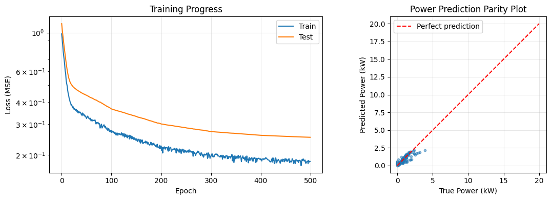
dP: R² = 0.9912
dT: R² = 0.6236
Power: R² = 0.7499
Compare Physics and Surrogate Models#
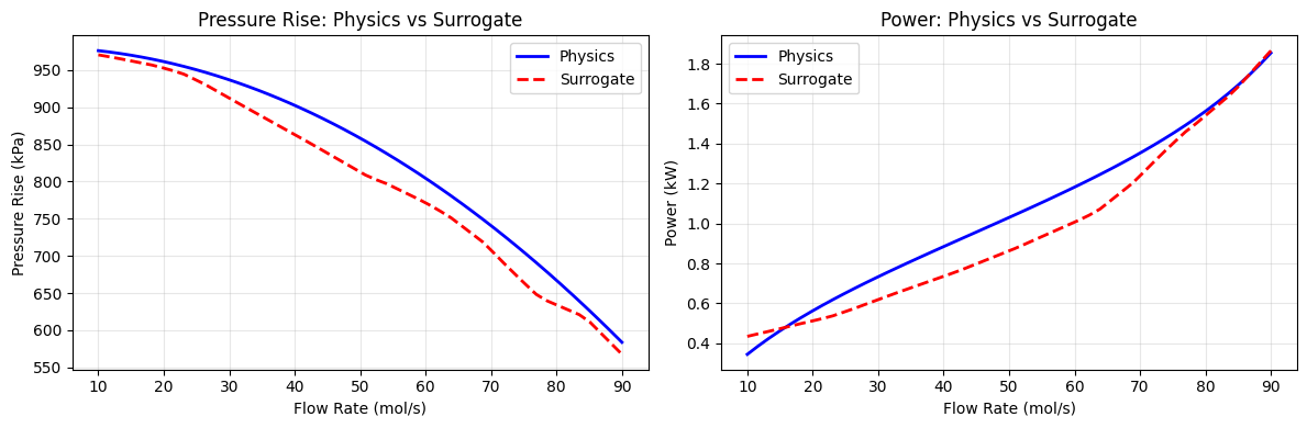
# Compare predictions across flow range
flow_range = jnp.linspace(10, 90, 50)
T_fixed, P_fixed, speed_fixed = 300.0, 101325.0, 1.0

physics_results = {'dP': [], 'power': []}
surrogate_results = {'dP': [], 'power': []}

for F in flow_range:
    inlet = make_stream({'water': float(F)}, T=T_fixed, P=P_fixed)

    _, info_phys = physics_pump(inlet, speed_fraction=speed_fixed)
    _, info_surr = surrogate_pump(inlet, speed_fraction=speed_fixed)

    physics_results['dP'].append(info_phys['dP'])
    physics_results['power'].append(info_phys['power'])
    surrogate_results['dP'].append(info_surr['dP'])
    surrogate_results['power'].append(info_surr['power'])

fig, axes = plt.subplots(1, 2, figsize=(12, 4))

axes[0].plot(flow_range, jnp.array(physics_results['dP'])/1000, 'b-', label='Physics', linewidth=2)
axes[0].plot(flow_range, jnp.array(surrogate_results['dP'])/1000, 'r--', label='Surrogate', linewidth=2)
axes[0].set_xlabel('Flow Rate (mol/s)')
axes[0].set_ylabel('Pressure Rise (kPa)')
axes[0].set_title('Pressure Rise: Physics vs Surrogate')
axes[0].legend()
axes[0].grid(True, alpha=0.3)

axes[1].plot(flow_range, jnp.array(physics_results['power'])/1000, 'b-', label='Physics', linewidth=2)
axes[1].plot(flow_range, jnp.array(surrogate_results['power'])/1000, 'r--', label='Surrogate', linewidth=2)
axes[1].set_xlabel('Flow Rate (mol/s)')
axes[1].set_ylabel('Power (kW)')
axes[1].set_title('Power: Physics vs Surrogate')
axes[1].legend()
axes[1].grid(True, alpha=0.3)

plt.tight_layout()
plt.show()
4. Dynamic Surrogate Pump Model#
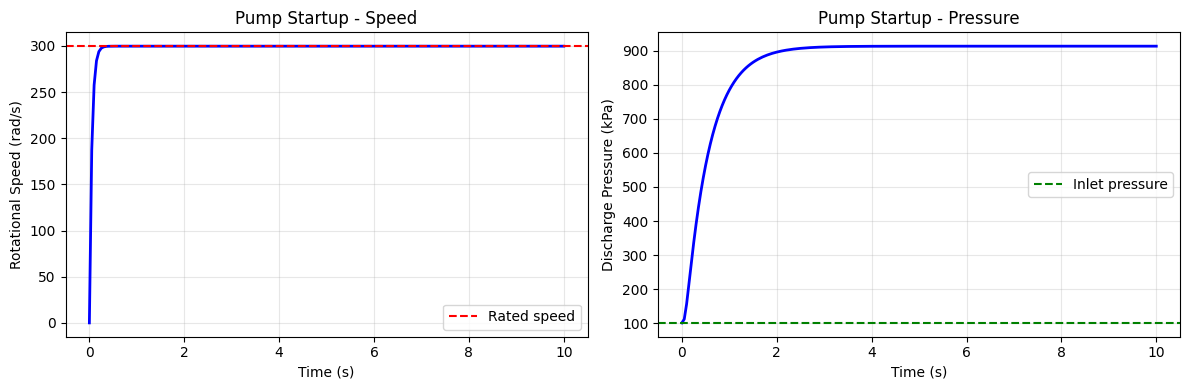
Now let’s create a dynamic pump model that can simulate startup transients.
The dynamic pump has state variables:
omega: Rotational speed (rad/s)
P_discharge: Discharge pressure (Pa)
Dynamics:
Motor inertia: \(J \frac{d\omega}{dt} = \tau_{motor} - \tau_{load}\)
Pressure dynamics: \(\tau_P \frac{dP}{dt} = P_{ss}(\omega, Q) - P\)
class DynamicSurrogatePump(DynamicUnitBase):
    """Dynamic pump with neural network steady-state surrogate.

    State variables:
        - omega: Rotational speed (rad/s)
        - P_discharge: Discharge pressure (Pa)

    The neural network predicts steady-state behavior, while
    the dynamics capture motor inertia and pressure lag.
    """

    def __init__(
        self,
        nn_params,
        input_scale,
        output_scale,
        omega_rated: float = 300.0,  # Rated speed (rad/s)
        J: float = 0.5,              # Motor inertia (kg·m²)
        tau_P: float = 0.5,          # Pressure time constant (s)
        K_motor: float = 10.0,       # Motor torque constant
        name: str | None = None,
    ):
        self.nn_params = nn_params
        self.input_mean, self.input_std = input_scale
        self.output_mean, self.output_std = output_scale
        self.omega_rated = omega_rated
        self.J = J
        self.tau_P = tau_P
        self.K_motor = K_motor

        super().__init__(name=name)

    def _build_state_spec(self) -> StateSpec:
        """Define state variables."""
        return StateSpec([
            StateVar(
                name="omega",
                category="generic",
                units="rad/s",
                description="Rotational speed",
                bounds=(0.0, None),
                scale=self.omega_rated,
                initial_value=0.0,
            ),
            StateVar(
                name="P_discharge",
                category="pressure",
                units="Pa",
                description="Discharge pressure",
                bounds=(0.0, None),
                scale=200000.0,
                initial_value=101325.0,
            ),
        ])

    def _predict_steady_state(self, F_total, T_in, P_in, speed_frac):
        """Neural network prediction of steady-state."""
        features = jnp.array([F_total, T_in, P_in, speed_frac])
        x_norm = (features - self.input_mean) / (self.input_std + 1e-8)
        y_norm = mlp_forward(self.nn_params, x_norm)
        outputs = y_norm * self.output_std + self.output_mean
        return outputs  # [dP, dT, power]

    def _derivatives(
        self,
        t: jnp.ndarray,
        state: StateVector,
        inputs: dict,
    ) -> jnp.ndarray:
        """Compute state derivatives."""
        omega = state["omega"]
        P_discharge = state["P_discharge"]

        # Get inlet conditions
        inlet = inputs.get("inlet") or list(inputs.values())[0]
        F_total = total_flow(inlet)
        T_in = inlet["T"]
        P_in = inlet["P"]

        # Speed setpoint from params (normalized)
        omega_sp = self.params.get("omega_setpoint", self.omega_rated)
        speed_frac = omega / self.omega_rated

        # Neural network predicts steady-state at current speed
        ss_outputs = self._predict_steady_state(F_total, T_in, P_in, speed_frac)
        dP_ss = jnp.maximum(ss_outputs[0], 0.0)
        power_ss = jnp.maximum(ss_outputs[2], 0.0)

        # Target discharge pressure
        P_target = P_in + dP_ss

        # Motor dynamics: J * d(omega)/dt = tau_motor - tau_load
        # Simplified: tau_motor proportional to error from setpoint
        # tau_load proportional to power / omega
        tau_motor = self.K_motor * (omega_sp - omega)
        tau_load = power_ss / (omega + 1e-6)
        d_omega = (tau_motor - tau_load) / self.J

        # Pressure dynamics: first-order lag
        d_P = (P_target - P_discharge) / self.tau_P

        return jnp.array([d_omega, d_P])

    def _outputs(
        self,
        t: jnp.ndarray,
        state: StateVector,
        inputs: dict,
    ) -> dict:
        """Compute outlet stream from state."""
        omega = state["omega"]
        P_discharge = state["P_discharge"]

        inlet = inputs.get("inlet") or list(inputs.values())[0]
        F_total = total_flow(inlet)
        T_in = inlet["T"]
        P_in = inlet["P"]

        speed_frac = omega / self.omega_rated

        # Get temperature rise from NN
        ss_outputs = self._predict_steady_state(F_total, T_in, P_in, speed_frac)
        dT = ss_outputs[1]

        # Create outlet
        outlet_flows = get_flows(inlet)
        outlet = make_stream(outlet_flows, T_in + dT, P_discharge)

        return {"outlet": outlet}

    def initial_state(
        self,
        inputs: dict,
        params: dict | None = None,
    ) -> jnp.ndarray:
        """Initialize at rest with inlet pressure."""
        inlet = inputs.get("inlet") or list(inputs.values())[0]
        return jnp.array([0.0, inlet["P"]])  # omega=0, P=P_inlet


# Create dynamic surrogate pump
dynamic_pump = DynamicSurrogatePump(
    nn_params=nn_params,
    input_scale=input_scale,
    output_scale=output_scale,
    name="pump",
)

print(f"Dynamic pump states: {dynamic_pump.state_spec().names}")
print(f"Number of states: {dynamic_pump.state_spec().n_states}")
Dynamic pump states: ['omega', 'P_discharge']
Number of states: 2
Simulate Pump Startup#
# Create inlet stream
inlet = make_stream({'water': 50.0}, T=300.0, P=101325.0)

# Simulate startup
result = integrate_unit(
    dynamic_pump,
    inputs={"inlet": inlet},
    t_span=(0.0, 10.0),  # 10 seconds
    method="RK4",
    n_steps=200,
)

print(f"Initial state: omega={result.trajectory.y[0, 0]:.1f} rad/s, P={result.trajectory.y[0, 1]/1000:.1f} kPa")
print(f"Final state:   omega={result.y_final[0]:.1f} rad/s, P={result.y_final[1]/1000:.1f} kPa")
Initial state: omega=0.0 rad/s, P=101.3 kPa
Final state:   omega=299.7 rad/s, P=912.8 kPa
# Plot startup dynamics
fig, axes = plt.subplots(1, 2, figsize=(12, 4))

# Speed profile
axes[0].plot(result.trajectory.t, result.trajectory.y[:, 0], 'b-', linewidth=2)
axes[0].axhline(dynamic_pump.omega_rated, color='r', linestyle='--', label='Rated speed')
axes[0].set_xlabel('Time (s)')
axes[0].set_ylabel('Rotational Speed (rad/s)')
axes[0].set_title('Pump Startup - Speed')
axes[0].legend()
axes[0].grid(True, alpha=0.3)

# Pressure profile
axes[1].plot(result.trajectory.t, result.trajectory.y[:, 1]/1000, 'b-', linewidth=2)
axes[1].axhline(inlet['P']/1000, color='g', linestyle='--', label='Inlet pressure')
axes[1].set_xlabel('Time (s)')
axes[1].set_ylabel('Discharge Pressure (kPa)')
axes[1].set_title('Pump Startup - Pressure')
axes[1].legend()
axes[1].grid(True, alpha=0.3)

plt.tight_layout()
plt.show()
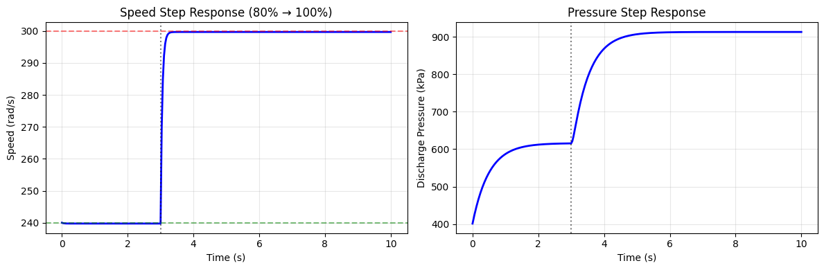
Speed Step Response#
def simulate_speed_step(pump, inlet, omega_initial, omega_final, t_step, t_total):
    """Simulate pump response to speed setpoint change."""

    # Phase 1: Run at initial speed until step time
    pump._params["omega_setpoint"] = omega_initial
    y0 = jnp.array([omega_initial, inlet["P"] + 300000.0])  # Start near steady-state

    result1 = integrate_unit(
        pump,
        inputs={"inlet": inlet},
        t_span=(0.0, t_step),
        y0=y0,
        method="RK4",
        n_steps=100,
    )

    # Phase 2: Step to new speed
    pump._params["omega_setpoint"] = omega_final

    result2 = integrate_unit(
        pump,
        inputs={"inlet": inlet},
        t_span=(t_step, t_total),
        y0=result1.y_final,
        method="RK4",
        n_steps=200,
    )

    # Combine results
    t_combined = jnp.concatenate([result1.trajectory.t, result2.trajectory.t[1:]])
    y_combined = jnp.vstack([result1.trajectory.y, result2.trajectory.y[1:]])

    return t_combined, y_combined, t_step


# Simulate step from 80% to 100% speed
inlet = make_stream({'water': 50.0}, T=300.0, P=101325.0)
omega_initial = 0.8 * dynamic_pump.omega_rated
omega_final = 1.0 * dynamic_pump.omega_rated

t_combined, y_combined, t_step = simulate_speed_step(
    dynamic_pump, inlet, omega_initial, omega_final, t_step=3.0, t_total=10.0
)

fig, axes = plt.subplots(1, 2, figsize=(12, 4))

# Speed response
axes[0].plot(t_combined, y_combined[:, 0], 'b-', linewidth=2)
axes[0].axvline(t_step, color='k', linestyle=':', alpha=0.5, label='Step input')
axes[0].axhline(omega_initial, color='g', linestyle='--', alpha=0.5)
axes[0].axhline(omega_final, color='r', linestyle='--', alpha=0.5)
axes[0].set_xlabel('Time (s)')
axes[0].set_ylabel('Speed (rad/s)')
axes[0].set_title('Speed Step Response (80% → 100%)')
axes[0].grid(True, alpha=0.3)

# Pressure response
axes[1].plot(t_combined, y_combined[:, 1]/1000, 'b-', linewidth=2)
axes[1].axvline(t_step, color='k', linestyle=':', alpha=0.5, label='Step input')
axes[1].set_xlabel('Time (s)')
axes[1].set_ylabel('Discharge Pressure (kPa)')
axes[1].set_title('Pressure Step Response')
axes[1].grid(True, alpha=0.3)

plt.tight_layout()
plt.show()
5. Gradient-Based Optimization Through Surrogate#
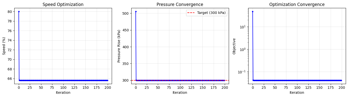
One key advantage of differentiable surrogates is the ability to compute gradients for optimization. Let’s optimize the pump speed to minimize energy while meeting a pressure target.
# Static optimization: find optimal speed for target pressure
# Note: We use the physics pump here for accurate optimization results.
# The surrogate would work similarly once better trained (R² > 0.9 on dP).

def objective(speed_frac, inlet, target_dP):
    """Objective: achieve target pressure with minimum power."""
    _, info = physics_pump(inlet, speed_fraction=speed_frac)

    # Strong penalty for missing pressure target (primary constraint)
    pressure_error = 100.0 * (info['dP'] - target_dP)**2 / target_dP**2

    # Small power cost (secondary objective: minimize energy)
    power_cost = 0.0001 * info['power']

    return pressure_error + power_cost


# Target: 300 kPa pressure rise
inlet = make_stream({'water': 50.0}, T=300.0, P=101325.0)
target_dP = 300000.0  # Pa

# At F=50 mol/s, physics pump gives ~858 kPa at 100% speed
# Theory: optimal is ~66% speed for 300 kPa (gradient changes sign at ~66%)

# Gradient descent optimization
# Note: gradients can be large (>700), so use small learning rate
speed = jnp.array(0.8)  # Initial guess
learning_rate = 0.0002  # Very small LR due to large gradients
history = []

for i in range(200):
    obj_val = objective(speed, inlet, target_dP)
    grad_val = grad(objective)(speed, inlet, target_dP)

    _, info = physics_pump(inlet, speed_fraction=float(speed))
    history.append({
        'speed': float(speed),
        'objective': float(obj_val),
        'dP': float(info['dP']),
        'power': float(info['power']),
    })

    speed = speed - learning_rate * grad_val
    speed = jnp.clip(speed, 0.5, 1.0)  # Physical bounds

print(f"Optimal speed: {history[-1]['speed']*100:.1f}%")
print(f"Pressure rise: {history[-1]['dP']/1000:.1f} kPa (target: {target_dP/1000:.0f} kPa)")
print(f"Power: {history[-1]['power']/1000:.2f} kW")
Optimal speed: 65.6%
Pressure rise: 300.0 kPa (target: 300 kPa)
Power: 0.42 kW
# Plot optimization progress
fig, axes = plt.subplots(1, 3, figsize=(14, 4))

iterations = range(len(history))

axes[0].plot(iterations, [h['speed']*100 for h in history], 'b-o', markersize=3)
axes[0].set_xlabel('Iteration')
axes[0].set_ylabel('Speed (%)')
axes[0].set_title('Speed Optimization')
axes[0].grid(True, alpha=0.3)

axes[1].plot(iterations, [h['dP']/1000 for h in history], 'b-o', markersize=3)
axes[1].axhline(target_dP/1000, color='r', linestyle='--', label=f'Target ({target_dP/1000:.0f} kPa)')
axes[1].set_xlabel('Iteration')
axes[1].set_ylabel('Pressure Rise (kPa)')
axes[1].set_title('Pressure Convergence')
axes[1].legend()
axes[1].grid(True, alpha=0.3)

axes[2].semilogy(iterations, [h['objective'] for h in history], 'b-o', markersize=3)
axes[2].set_xlabel('Iteration')
axes[2].set_ylabel('Objective')
axes[2].set_title('Optimization Convergence')
axes[2].grid(True, alpha=0.3)

plt.tight_layout()
plt.show()
6. Dynamic Optimization#
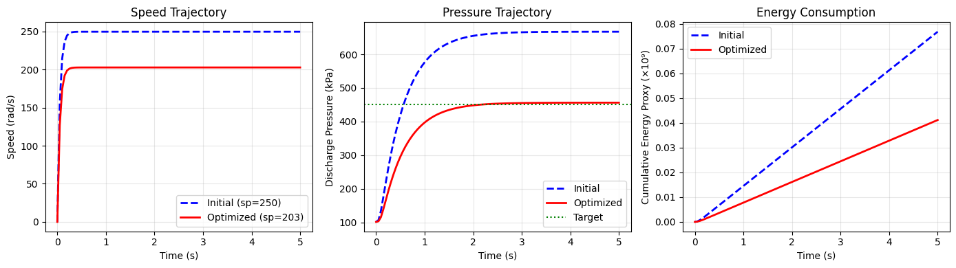
Optimize pump startup trajectory to minimize energy while reaching target pressure quickly.
def dynamic_objective(omega_setpoint, inlet, target_P, t_final=5.0):
    """Objective for dynamic optimization.

    Minimize: settling time + integral of speed^3 (proxy for energy)
    Subject to: reach target pressure
    """
    # Create pump with given setpoint
    pump = DynamicSurrogatePump(
        nn_params=nn_params,
        input_scale=input_scale,
        output_scale=output_scale,
    )
    pump._params["omega_setpoint"] = omega_setpoint

    # Simulate
    result = integrate_unit(
        pump,
        inputs={"inlet": inlet},
        t_span=(0.0, t_final),
        method="RK4",
        n_steps=100,
    )

    # Terminal pressure error
    P_final = result.y_final[1]
    pressure_error = (P_final - target_P)**2 / target_P**2

    # Energy proxy: integral of omega^3 (power ~ omega^3)
    omega_traj = result.trajectory.y[:, 0]
    energy_proxy = jnp.mean(omega_traj**3) / (pump.omega_rated**3)

    return pressure_error * 10 + energy_proxy * 0.1


# Optimize omega setpoint
inlet = make_stream({'water': 50.0}, T=300.0, P=101325.0)
target_P = inlet['P'] + 350000.0  # Target discharge pressure

omega_sp = jnp.array(250.0)  # Initial guess
learning_rate = 50.0
dynamic_history = []

print("Optimizing pump speed setpoint...")
for i in range(30):
    obj_val = dynamic_objective(omega_sp, inlet, target_P)
    grad_val = grad(dynamic_objective)(omega_sp, inlet, target_P)

    dynamic_history.append({
        'omega_sp': float(omega_sp),
        'objective': float(obj_val),
    })

    omega_sp = omega_sp - learning_rate * grad_val
    omega_sp = jnp.clip(omega_sp, 100.0, 400.0)

    if i % 10 == 0:
        print(f"  Iter {i}: omega_sp={omega_sp:.1f} rad/s, obj={obj_val:.6f}")

print(f"\nOptimal speed setpoint: {dynamic_history[-1]['omega_sp']:.1f} rad/s")
Optimizing pump speed setpoint...
Iter 0: omega_sp=244.5 rad/s, obj=2.346596
Iter 10: omega_sp=220.4 rad/s, obj=0.519516
Iter 20: omega_sp=206.0 rad/s, obj=0.069089
Optimal speed setpoint: 203.0 rad/s
# Compare initial vs optimized trajectories
omega_initial = 250.0
omega_optimal = dynamic_history[-1]['omega_sp']

fig, axes = plt.subplots(1, 3, figsize=(14, 4))

for omega_sp, label, style in [(omega_initial, 'Initial', 'b--'), (omega_optimal, 'Optimized', 'r-')]:
    pump = DynamicSurrogatePump(
        nn_params=nn_params,
        input_scale=input_scale,
        output_scale=output_scale,
    )
    pump._params["omega_setpoint"] = omega_sp

    result = integrate_unit(
        pump,
        inputs={"inlet": inlet},
        t_span=(0.0, 5.0),
        method="RK4",
        n_steps=100,
    )

    axes[0].plot(result.trajectory.t, result.trajectory.y[:, 0], style,
                 label=f'{label} (sp={omega_sp:.0f})', linewidth=2)
    axes[1].plot(result.trajectory.t, result.trajectory.y[:, 1]/1000, style,
                 label=label, linewidth=2)

    # Energy proxy
    energy = jnp.cumsum(result.trajectory.y[:, 0]**3) * (5.0/100)
    axes[2].plot(result.trajectory.t, energy / 1e9, style, label=label, linewidth=2)

axes[0].set_xlabel('Time (s)')
axes[0].set_ylabel('Speed (rad/s)')
axes[0].set_title('Speed Trajectory')
axes[0].legend()
axes[0].grid(True, alpha=0.3)

axes[1].axhline(target_P/1000, color='g', linestyle=':', label='Target')
axes[1].set_xlabel('Time (s)')
axes[1].set_ylabel('Discharge Pressure (kPa)')
axes[1].set_title('Pressure Trajectory')
axes[1].legend()
axes[1].grid(True, alpha=0.3)

axes[2].set_xlabel('Time (s)')
axes[2].set_ylabel('Cumulative Energy Proxy (×10⁹)')
axes[2].set_title('Energy Consumption')
axes[2].legend()
axes[2].grid(True, alpha=0.3)

plt.tight_layout()
plt.show()
7. Using Surrogate in a Flowsheet#
Finally, let’s demonstrate using the static surrogate pump within a flowsheet.
from difflow import Flowsheet, Unit

# Create a simple flowsheet: Feed → Pump → Heater → Product

# Wrap surrogate pump for flowsheet interface
def pump_operation(inlet, speed_fraction=1.0):
    """Wrapper for surrogate pump in flowsheet."""
    return surrogate_pump(inlet, speed_fraction=speed_fraction)


# Create heater (needs thermo for enthalpy calculations)
# For simplicity, we'll create a minimal heater that just adds heat
def simple_heater(inlet, T_out=350.0):
    """Simple heater that sets outlet temperature."""
    outlet_flows = get_flows(inlet)
    outlet = make_stream(outlet_flows, T_out, inlet['P'])

    # Estimate duty
    Cp = 75.0  # J/mol/K
    F_total = total_flow(inlet)
    Q = F_total * Cp * (T_out - inlet['T'])

    return outlet, {'Q': Q, 'T_out': T_out}


# Build flowsheet
fs = Flowsheet(species_order=['water'])

# Add feed
feed = make_stream({'water': 50.0}, T=290.0, P=101325.0)
fs.add_feed('feed', feed)

# Add pump
fs.add_unit(Unit(
    name='pump',
    operation=pump_operation,
    inlet_names=['feed'],
    outlet_names=['pumped'],
    params={'speed_fraction': 0.9},
))

# Add heater
fs.add_unit(Unit(
    name='heater',
    operation=simple_heater,
    inlet_names=['pumped'],
    outlet_names=['product'],
    params={'T_out': 350.0},
))

# Solve flowsheet
streams = fs.solve()

# Get unit info by re-running the operations on the solved streams
_, pump_info = surrogate_pump(streams['feed'], speed_fraction=0.9)
_, heater_info = simple_heater(streams['pumped'], T_out=350.0)

print("Flowsheet Results:")
print(f"\nFeed:")
print(f"  F = {total_flow(streams['feed']):.1f} mol/s")
print(f"  T = {streams['feed']['T']:.1f} K")
print(f"  P = {streams['feed']['P']/1000:.1f} kPa")

print(f"\nAfter Pump:")
print(f"  F = {total_flow(streams['pumped']):.1f} mol/s")
print(f"  T = {streams['pumped']['T']:.2f} K")
print(f"  P = {streams['pumped']['P']/1000:.1f} kPa")
print(f"  Power = {pump_info['power']/1000:.2f} kW")

print(f"\nProduct:")
print(f"  F = {total_flow(streams['product']):.1f} mol/s")
print(f"  T = {streams['product']['T']:.1f} K")
print(f"  P = {streams['product']['P']/1000:.1f} kPa")
print(f"  Heater duty = {heater_info['Q']/1000:.2f} kW")
Flowsheet Results:

Feed:
  F = 50.0 mol/s
  T = 290.0 K
  P = 101.3 kPa

After Pump:
  F = 50.0 mol/s
  T = 290.05 K
  P = 767.2 kPa
  Power = 0.74 kW

Product:
  F = 50.0 mol/s
  T = 350.0 K
  P = 767.2 kPa
  Heater duty = 224.79 kW
Flowsheet Optimization with Surrogate#
def flowsheet_cost(speed_fraction, T_heater, feed):
    """Total operating cost: pump power + heater duty."""
    # Pump
    pumped, pump_info = surrogate_pump(feed, speed_fraction=speed_fraction)

    # Heater
    product, heater_info = simple_heater(pumped, T_out=T_heater)

    # Cost: electricity for pump ($0.10/kWh) + steam for heater ($0.02/kWh)
    pump_cost = pump_info['power'] / 1000 * 0.10  # $/h
    heater_cost = jnp.maximum(heater_info['Q'], 0.0) / 1000 * 0.02  # $/h

    # Constraint: final pressure must be > 300 kPa
    pressure_penalty = jnp.maximum(300000.0 - pumped['P'], 0.0)**2 / 1e10

    return pump_cost + heater_cost + pressure_penalty


# Optimize pump speed and heater temperature
feed = make_stream({'water': 50.0}, T=290.0, P=101325.0)

# Use manual gradient descent (could use scipy.optimize with JAX gradients)
speed = jnp.array(0.9)
T_heat = jnp.array(350.0)
lr_speed, lr_T = 0.1, 10.0

print("Optimizing flowsheet...")
for i in range(50):
    cost = flowsheet_cost(speed, T_heat, feed)
    grad_speed = grad(flowsheet_cost, argnums=0)(speed, T_heat, feed)
    grad_T = grad(flowsheet_cost, argnums=1)(speed, T_heat, feed)

    speed = jnp.clip(speed - lr_speed * grad_speed, 0.5, 1.0)
    T_heat = jnp.clip(T_heat - lr_T * grad_T, 300.0, 400.0)

    if i % 10 == 0:
        print(f"  Iter {i}: speed={speed*100:.1f}%, T_heat={T_heat:.1f} K, cost=${cost:.4f}/h")

print(f"\nOptimal: speed={speed*100:.1f}%, T_heater={T_heat:.1f} K")
print(f"Minimum cost: ${flowsheet_cost(speed, T_heat, feed):.4f}/h")
Optimizing flowsheet...
Iter 0: speed=89.0%, T_heat=349.2 K, cost=$4.5700/h
Iter 10: speed=81.2%, T_heat=341.8 K, cost=$4.0009/h
Iter 20: speed=69.4%, T_heat=334.2 K, cost=$3.4234/h
Iter 30: speed=77.7%, T_heat=326.8 K, cost=$2.8491/h
Iter 40: speed=64.8%, T_heat=319.2 K, cost=$2.2905/h
Optimal: speed=62.2%, T_heater=312.5 K
Minimum cost: $1.7241/h
Summary#
This notebook demonstrated:
Physics-based pump model as ground truth for generating training data
Static surrogate pump using a neural network to predict:
Pressure rise
Temperature rise
Power consumption
Training the surrogate with MSE loss and mini-batch SGD
Dynamic surrogate pump implementing
DynamicUnitBasewith:Rotational speed dynamics (motor inertia)
Pressure dynamics (first-order lag)
NN-based steady-state prediction
Gradient-based optimization through both static and dynamic surrogates
Flowsheet integration showing surrogates work seamlessly with difflow
Key Takeaways#
Surrogates follow the same interface as physics models:
outlet, info = unit(inlet, **params)Full JAX differentiability enables gradient-based optimization
Dynamic surrogates combine NN steady-state predictions with physics-based dynamics
Training data can come from detailed models, experiments, or process simulators