
Heat Exchanger Examples#
This notebook demonstrates the heat exchanger unit operations in difflow:
Simple Examples: Heaters and coolers with utilities
Two-Stream Heat Exchangers: Counter-current, co-current, and cross-flow
Design and Sizing: LMTD and effectiveness-NTU methods
Advanced Example: Reactor with feed preheating (heat integration)
Optimization: Minimize utility cost with gradient-based optimization
import jax
import jax.numpy as jnp
import matplotlib.pyplot as plt

from difflow import (
    make_stream,
    Heater, HeaterParams,
    Cooler, CoolerParams,
    CounterCurrentHX, CoCurrentHX, CrossFlowHX, HeatExchangerParams,
    log_mean_temperature_difference,
    design_heat_exchanger,
    size_heat_exchanger,
    CSTR, CSTRParams,
    IdealThermo, SpeciesData,
)

# Enable float64 for better numerical precision
jax.config.update('jax_enable_x64', True)
WARNING:2026-01-10 19:35:14,721:jax._src.xla_bridge:852: An NVIDIA GPU may be present on this machine, but a CUDA-enabled jaxlib is not installed. Falling back to cpu.
1. Simple Examples: Heaters and Coolers#
Single-stream heat exchangers with utilities (steam, cooling water, etc.)
1.1 Heater with Specified Duty#
# Create a process stream
feed = make_stream({"methanol": 10.0, "water": 5.0}, T=300.0, P=101325.0)

# Heater with 50 kW duty
# Cp = 75 J/(mol·K) is typical for organic liquids
heater = Heater(HeaterParams(duty=50000.0, Cp=75.0))
heated, info = heater(feed)

print("Heater with Specified Duty")
print(f"  Inlet temperature:  {float(info['T_in']):.1f} K")
print(f"  Outlet temperature: {float(info['T_out']):.1f} K")
print(f"  Heat duty:          {float(info['Q'])/1000:.1f} kW")
print(f"  Temperature rise:   {float(info['T_out'] - info['T_in']):.1f} K")
Heater with Specified Duty
  Inlet temperature:  300.0 K
  Outlet temperature: 344.4 K
  Heat duty:          50.0 kW
  Temperature rise:   44.4 K
1.2 Heater with Specified Outlet Temperature#
# Heat feed to 350 K
heater = Heater(HeaterParams(T_out=350.0, Cp=75.0))
heated, info = heater(feed)

print("Heater with Specified Outlet Temperature")
print(f"  Target temperature: 350.0 K")
print(f"  Required duty:      {float(info['Q'])/1000:.2f} kW")
Heater with Specified Outlet Temperature
  Target temperature: 350.0 K
  Required duty:      56.25 kW
1.3 Heater Rating Mode (with UA and utility temperature)#
# Heater with steam at 423 K (150°C, ~5 bar steam)
# UA = 2000 W/K (typical for shell-and-tube)
heater = Heater(HeaterParams(UA=2000.0, T_utility=423.0, Cp=75.0))
heated, info = heater(feed)

print("Heater Rating Mode")
print(f"  Steam temperature:  {423.0} K ({423-273:.0f}°C)")
print(f"  UA:                 {2000} W/K")
print(f"  Outlet temperature: {float(info['T_out']):.1f} K")
print(f"  Heat duty:          {float(info['Q'])/1000:.2f} kW")
print(f"  LMTD:               {float(info['LMTD']):.1f} K")
Heater Rating Mode
  Steam temperature:  423.0 K (150°C)
  UA:                 2000 W/K
  Outlet temperature: 402.2 K
  Heat duty:          114.99 kW
  LMTD:               57.5 K
1.4 Cooler Example#
# Hot stream from reactor
hot_product = make_stream({"product": 8.0, "byproduct": 2.0}, T=420.0, P=101325.0)

# Cool to 320 K using cooling water (utility at 298 K)
cooler = Cooler(CoolerParams(T_out=320.0, T_utility=298.0, Cp=80.0))
cooled, info = cooler(hot_product)

print("Cooler Example")
print(f"  Inlet temperature:  {float(info['T_in']):.1f} K")
print(f"  Outlet temperature: {float(info['T_out']):.1f} K")
print(f"  Heat removed:       {float(info['Q'])/1000:.2f} kW")
print(f"  LMTD:               {float(info['LMTD']):.1f} K")
print(f"  Required UA:        {float(info['UA_required']):.1f} W/K")
Cooler Example
  Inlet temperature:  420.0 K
  Outlet temperature: 320.0 K
  Heat removed:       80.00 kW
  LMTD:               58.4 K
  Required UA:        1370.4 W/K
2. Two-Stream Heat Exchangers#
Process-to-process heat exchange for heat integration.
2.1 Counter-Current Heat Exchanger#
# Hot product stream leaving reactor
hot_stream = make_stream({"product": 10.0}, T=450.0, P=101325.0)

# Cold feed stream entering process
cold_stream = make_stream({"feed": 10.0}, T=300.0, P=101325.0)

# Counter-current heat exchanger
hx = CounterCurrentHX(HeatExchangerParams(
    UA=1500.0,      # W/K
    Cp_hot=75.0,    # J/(mol·K)
    Cp_cold=75.0,
))

hot_out, cold_out, info = hx(hot_stream, cold_stream)

print("Counter-Current Heat Exchanger")
print(f"  Hot side:  {float(info['T_hot_in']):.1f} K → {float(info['T_hot_out']):.1f} K")
print(f"  Cold side: {float(info['T_cold_in']):.1f} K → {float(info['T_cold_out']):.1f} K")
print(f"  Heat transferred: {float(info['Q'])/1000:.2f} kW")
print(f"  Effectiveness:    {float(info['effectiveness']):.3f}")
print(f"  NTU:              {float(info['NTU']):.2f}")
print(f"  LMTD:             {float(info['LMTD']):.1f} K")
print(f"  Approach temp:    {float(info['approach']):.1f} K")
Counter-Current Heat Exchanger
  Hot side:  450.0 K → 350.0 K
  Cold side: 300.0 K → 400.0 K
  Heat transferred: 75.00 kW
  Effectiveness:    0.667
  NTU:              2.00
  LMTD:             50.0 K
  Approach temp:    50.0 K
2.2 Co-Current vs Counter-Current Comparison#
# Compare at same UA
UA_values = jnp.linspace(500, 5000, 20)

Q_counter = []
Q_co = []
eps_counter = []
eps_co = []

for UA in UA_values:
    # Counter-current
    hx_counter = CounterCurrentHX(HeatExchangerParams(Cp_hot=75.0, Cp_cold=75.0))
    _, _, info_counter = hx_counter(hot_stream, cold_stream, UA=float(UA))
    Q_counter.append(float(info_counter['Q']))
    eps_counter.append(float(info_counter['effectiveness']))

    # Co-current
    hx_co = CoCurrentHX(HeatExchangerParams(Cp_hot=75.0, Cp_cold=75.0))
    _, _, info_co = hx_co(hot_stream, cold_stream, UA=float(UA))
    Q_co.append(float(info_co['Q']))
    eps_co.append(float(info_co['effectiveness']))

fig, axes = plt.subplots(1, 2, figsize=(12, 4))

axes[0].plot(UA_values, jnp.array(Q_counter)/1000, 'b-', label='Counter-current', linewidth=2)
axes[0].plot(UA_values, jnp.array(Q_co)/1000, 'r--', label='Co-current', linewidth=2)
axes[0].set_xlabel('UA (W/K)')
axes[0].set_ylabel('Heat Duty (kW)')
axes[0].set_title('Heat Transfer vs UA')
axes[0].legend()
axes[0].grid(True, alpha=0.3)

axes[1].plot(UA_values, eps_counter, 'b-', label='Counter-current', linewidth=2)
axes[1].plot(UA_values, eps_co, 'r--', label='Co-current', linewidth=2)
axes[1].axhline(y=0.5, color='gray', linestyle=':', label='ε = 0.5 limit (co-current)')
axes[1].set_xlabel('UA (W/K)')
axes[1].set_ylabel('Effectiveness')
axes[1].set_title('Effectiveness vs UA')
axes[1].legend()
axes[1].grid(True, alpha=0.3)

plt.tight_layout()
plt.show()

print("\nNote: Counter-current always achieves higher effectiveness for the same UA.")
print("Co-current is limited to ε ≤ 0.5 for balanced flows (Cr = 1).")
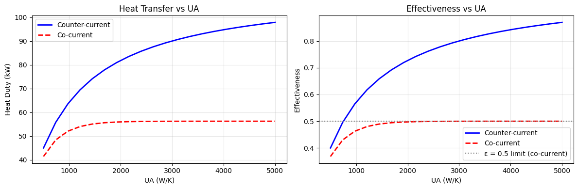
Note: Counter-current always achieves higher effectiveness for the same UA.
Co-current is limited to ε ≤ 0.5 for balanced flows (Cr = 1).
# Compare all flow configurations
UA_range = jnp.linspace(100, 5000, 30)

# Store results for each configuration
configs = {
    'Counter-current': {'hx': CounterCurrentHX, 'style': 'b-', 'linewidth': 2.5},
    'Cross (unmixed)': {'hx': lambda p: CrossFlowHX(p, mixing="both_unmixed"), 'style': 'g-', 'linewidth': 2},
    'Cross (Cmax mixed)': {'hx': lambda p: CrossFlowHX(p, mixing="cmax_mixed"), 'style': 'g--', 'linewidth': 1.5},
    'Cross (Cmin mixed)': {'hx': lambda p: CrossFlowHX(p, mixing="cmin_mixed"), 'style': 'g:', 'linewidth': 1.5},
    'Co-current': {'hx': CoCurrentHX, 'style': 'r-', 'linewidth': 2.5},
}

results_all = {name: {'Q': [], 'eps': [], 'NTU': []} for name in configs.keys()}

for UA in UA_range:
    params = HeatExchangerParams(Cp_hot=75.0, Cp_cold=75.0)

    for name, config in configs.items():
        hx = config['hx'](params)
        _, _, info = hx(hot_stream, cold_stream, UA=float(UA))
        results_all[name]['Q'].append(float(info['Q']))
        results_all[name]['eps'].append(float(info['effectiveness']))
        results_all[name]['NTU'].append(float(info['NTU']))

# Create comparison plots
fig, axes = plt.subplots(1, 2, figsize=(14, 5))

# Plot 1: Effectiveness vs NTU
for name, config in configs.items():
    axes[0].plot(results_all[name]['NTU'], results_all[name]['eps'],
                config['style'], label=name, linewidth=config['linewidth'])

axes[0].set_xlabel('NTU (Number of Transfer Units)', fontsize=11)
axes[0].set_ylabel('Effectiveness ε', fontsize=11)
axes[0].set_title('Heat Exchanger Effectiveness vs NTU\n(Balanced Flow: Cr = 1)', fontsize=12)
axes[0].legend(loc='lower right', fontsize=9)
axes[0].grid(True, alpha=0.3)
axes[0].set_xlim([0, 7])
axes[0].set_ylim([0, 1])

# Plot 2: Heat Duty vs UA
for name, config in configs.items():
    axes[1].plot(UA_range, jnp.array(results_all[name]['Q'])/1000,
                config['style'], label=name, linewidth=config['linewidth'])

axes[1].set_xlabel('UA (W/K)', fontsize=11)
axes[1].set_ylabel('Heat Duty (kW)', fontsize=11)
axes[1].set_title('Heat Transfer Rate vs UA\n(T_hot_in=450K, T_cold_in=300K)', fontsize=12)
axes[1].legend(loc='lower right', fontsize=9)
axes[1].grid(True, alpha=0.3)

plt.tight_layout()
plt.show()

print("\nKey Observations:")
print("1. Counter-current achieves highest effectiveness for any NTU")
print("2. Cross-flow (unmixed) performs between counter and co-current")
print("3. Mixed cross-flow configs are closer to counter-current performance")
print("4. Co-current is limited to ε = 0.5 for balanced flows (Cr = 1)")
print("5. All configurations converge to same heat duty at high UA (approach limit)")
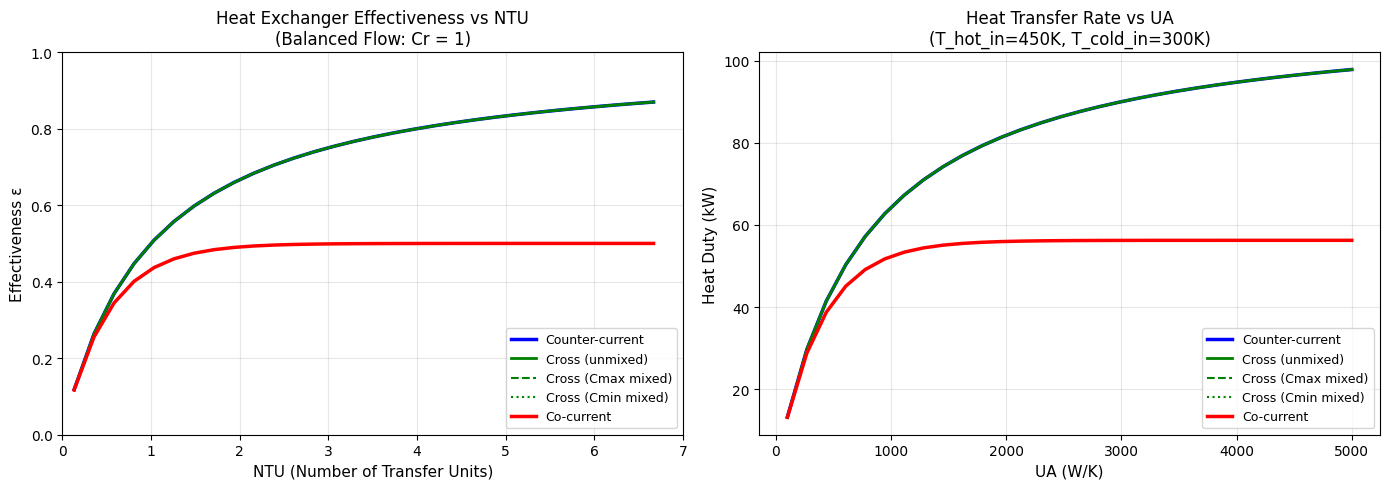
Key Observations:
1. Counter-current achieves highest effectiveness for any NTU
2. Cross-flow (unmixed) performs between counter and co-current
3. Mixed cross-flow configs are closer to counter-current performance
4. Co-current is limited to ε = 0.5 for balanced flows (Cr = 1)
5. All configurations converge to same heat duty at high UA (approach limit)
2.4 Flow Configuration Comparison#
Compare all available heat exchanger configurations to understand their relative performance.
# Compare all cross-flow configurations at same UA
UA_crossflow = 1500.0

mixing_configs = ["both_unmixed", "cmax_mixed", "cmin_mixed", "both_mixed"]
results = {}

for config in mixing_configs:
    hx_cross = CrossFlowHX(
        HeatExchangerParams(Cp_hot=75.0, Cp_cold=75.0),
        mixing=config
    )
    hot_out, cold_out, info = hx_cross(hot_stream, cold_stream, UA=UA_crossflow)
    results[config] = info

print("Cross-Flow Heat Exchanger Comparison (UA = 1500 W/K)")
print("="*65)
print(f"{'Configuration':<18} {'Q (kW)':<10} {'ε':<8} {'T_hot_out (K)':<15} {'T_cold_out (K)'}")
print("-"*65)

for config in mixing_configs:
    info = results[config]
    print(f"{config:<18} {float(info['Q'])/1000:<10.2f} {float(info['effectiveness']):<8.4f} "
          f"{float(info['T_hot_out']):<15.1f} {float(info['T_cold_out']):.1f}")

print("\nNotes:")
print("- Both unmixed is most common configuration (car radiators, finned-tube HX)")
print("- Mixed configurations allow better heat transfer but are less common")
print("- All cross-flow configs fall between counter-current and co-current effectiveness")
Cross-Flow Heat Exchanger Comparison (UA = 1500 W/K)
=================================================================
Configuration      Q (kW)     ε        T_hot_out (K)   T_cold_out (K)
-----------------------------------------------------------------
both_unmixed       75.00      0.6667   350.0           400.0
cmax_mixed         75.00      0.6667   350.0           400.0
cmin_mixed         75.00      0.6667   350.0           400.0
both_mixed         62.05      0.5516   367.3           382.7

Notes:
- Both unmixed is most common configuration (car radiators, finned-tube HX)
- Mixed configurations allow better heat transfer but are less common
- All cross-flow configs fall between counter-current and co-current effectiveness
2.3 Cross-Flow Heat Exchangers#
Cross-flow heat exchangers have fluids flowing perpendicular to each other. The effectiveness depends on whether each fluid can mix in its flow direction:
both_unmixed: Most common (car radiators, finned-tube HX)
cmax_mixed: Larger heat capacity stream mixed
cmin_mixed: Smaller heat capacity stream mixed
both_mixed: Both streams can mix (less common)
3. Heat Exchanger Design and Sizing#
Calculate required area from process specifications.
3.1 LMTD Method (Given Temperatures)#
# Design specifications
Q_design = 100000.0  # 100 kW
T_hot_in = 450.0     # K
T_hot_out = 380.0    # K
T_cold_in = 300.0    # K
T_cold_out = 360.0   # K
U = 500.0            # W/(m²·K) - typical for liquid-liquid

result = design_heat_exchanger(
    Q=jnp.array(Q_design),
    T_hot_in=jnp.array(T_hot_in),
    T_hot_out=jnp.array(T_hot_out),
    T_cold_in=jnp.array(T_cold_in),
    T_cold_out=jnp.array(T_cold_out),
    U=jnp.array(U),
    flow_config="counter_current",
)

print("LMTD Design Method")
print(f"  Heat duty:     {Q_design/1000:.1f} kW")
print(f"  Hot side:      {T_hot_in:.0f} K → {T_hot_out:.0f} K")
print(f"  Cold side:     {T_cold_in:.0f} K → {T_cold_out:.0f} K")
print(f"  U:             {U:.0f} W/(m²·K)")
print("\nResults:")
print(f"  LMTD:          {float(result['LMTD']):.1f} K")
print(f"  Required UA:   {float(result['UA']):.1f} W/K")
print(f"  Required Area: {float(result['A']):.2f} m²")
LMTD Design Method
  Heat duty:     100.0 kW
  Hot side:      450 K → 380 K
  Cold side:     300 K → 360 K
  U:             500 W/(m²·K)

Results:
  LMTD:          84.9 K
  Required UA:   1177.8 W/K
  Required Area: 2.36 m²
3.2 Effectiveness-NTU Method (Given Flow Rates)#
# Design from heat capacity rates
C_hot = 750.0   # W/K (10 mol/s × 75 J/mol·K)
C_cold = 600.0  # W/K (8 mol/s × 75 J/mol·K)

result = size_heat_exchanger(
    Q=jnp.array(50000.0),        # 50 kW
    T_hot_in=jnp.array(450.0),
    T_cold_in=jnp.array(300.0),
    C_hot=jnp.array(C_hot),
    C_cold=jnp.array(C_cold),
    U=jnp.array(500.0),
    flow_config="counter_current",
)

print("Effectiveness-NTU Sizing Method")
print(f"  Heat duty:       {50.0:.1f} kW")
print(f"  C_hot:           {C_hot:.0f} W/K")
print(f"  C_cold:          {C_cold:.0f} W/K")
print(f"  Cr (Cmin/Cmax):  {float(result['Cr']):.3f}")
print("\nResults:")
print(f"  Effectiveness:   {float(result['effectiveness']):.3f}")
print(f"  NTU:             {float(result['NTU']):.2f}")
print(f"  Required UA:     {float(result['UA']):.1f} W/K")
print(f"  Required Area:   {float(result['A']):.2f} m²")
print(f"  T_hot_out:       {float(result['T_hot_out']):.1f} K")
print(f"  T_cold_out:      {float(result['T_cold_out']):.1f} K")
Effectiveness-NTU Sizing Method
  Heat duty:       50.0 kW
  C_hot:           750 W/K
  C_cold:          600 W/K
  Cr (Cmin/Cmax):  0.800

Results:
  Effectiveness:   0.556
  NTU:             1.12
  Required UA:     669.4 W/K
  Required Area:   1.34 m²
  T_hot_out:       383.3 K
  T_cold_out:      383.3 K
4. Advanced Example: Reactor with Feed Preheating#
A common heat integration scenario: use hot reactor effluent to preheat cold feed.
# Define species for reactor
species_data = {
    "A": SpeciesData("A", MW=100.0, Cp_coeffs=(75.0, 0.0, 0.0, 0.0),
                     Hvap_coeffs=(35000.0, 0.38, 500.0),
                     antoine_coeffs=(10.0, 3000.0, -50.0), Hf=0.0),
    "B": SpeciesData("B", MW=100.0, Cp_coeffs=(80.0, 0.0, 0.0, 0.0),
                     Hvap_coeffs=(30000.0, 0.38, 450.0),
                     antoine_coeffs=(10.0, 2800.0, -40.0), Hf=-50000.0),
}
thermo = IdealThermo(species_data)

# Reaction kinetics: A → B (exothermic)
def rate_fn(C, T, params):
    k = params["k0"] * jnp.exp(-params["Ea"] / (8.314 * T))
    return jnp.array([k * C["A"]])

stoich = jnp.array([[-1.0], [+1.0]])  # A → B
rate_params = {"k0": jnp.array(1e8), "Ea": jnp.array(60000.0)}
4.1 Without Heat Integration (Base Case)#
# Cold feed at ambient temperature
cold_feed = make_stream({"A": 10.0, "B": 0.0}, T=298.0, P=101325.0)

# Heat feed to reactor temperature with steam
T_reactor = 400.0  # K
heater_feed = Heater(HeaterParams(T_out=T_reactor, Cp=75.0))
hot_feed, heater_info = heater_feed(cold_feed)

# Reactor (isothermal)
cstr = CSTR(
    CSTRParams(
        V=jnp.array(2.0),
        rate_fn=rate_fn,
        stoich=stoich,
        rate_params=rate_params,
        species_order=["A", "B"],
    ),
    thermo=thermo,
    mode="isothermal",
)

product, reactor_info = cstr(hot_feed, T_spec=T_reactor)

# Cool product to storage temperature
T_storage = 310.0  # K
cooler_product = Cooler(CoolerParams(T_out=T_storage, Cp=77.5))  # avg Cp
cooled_product, cooler_info = cooler_product(product)

print("Base Case: No Heat Integration")
print(f"\nFeed Heating:")
print(f"  Steam duty:        {float(heater_info['Q'])/1000:.2f} kW")
print(f"\nReactor:")
print(f"  Conversion:        {float(reactor_info['conversion']['A'])*100:.1f}%")
print(f"  Reactor heat duty: {float(reactor_info['Q'])/1000:.2f} kW (cooling needed)")
print(f"\nProduct Cooling:")
print(f"  Cooling duty:      {float(cooler_info['Q'])/1000:.2f} kW")
print(f"\nTotal Utilities:")
print(f"  Heating (steam):   {float(heater_info['Q'])/1000:.2f} kW")
print(f"  Cooling (CW):      {(float(cooler_info['Q']) + abs(float(reactor_info['Q'])))/1000:.2f} kW")
Base Case: No Heat Integration

Feed Heating:
  Steam duty:        76.50 kW

Reactor:
  Conversion:        93.6%
  Reactor heat duty: 4.77 kW (cooling needed)

Product Cooling:
  Cooling duty:      69.75 kW

Total Utilities:
  Heating (steam):   76.50 kW
  Cooling (CW):      74.52 kW
4.2 With Feed-Effluent Heat Exchanger (FEHE)#
def process_with_heat_integration(UA_fehe):
    """Simulate process with feed-effluent heat exchanger."""
    # Cold feed
    cold_feed = make_stream({"A": 10.0, "B": 0.0}, T=298.0, P=101325.0)

    # For this example, we'll use an iterative approach
    # In practice, this would be solved simultaneously

    # Initial guess for preheated feed temperature
    T_preheat = 340.0

    for _ in range(10):  # Simple iteration
        # Preheat feed in FEHE (estimate)
        preheated_feed = make_stream({"A": 10.0, "B": 0.0}, T=T_preheat, P=101325.0)

        # Additional heating to reactor temperature
        heater = Heater(HeaterParams(T_out=T_reactor, Cp=75.0))
        hot_feed, heater_info = heater(preheated_feed)

        # Reactor
        product, reactor_info = cstr(hot_feed, T_spec=T_reactor)

        # FEHE: hot product preheats cold feed
        fehe = CounterCurrentHX(HeatExchangerParams(
            UA=UA_fehe,
            Cp_hot=77.5,  # Product (mix of A and B)
            Cp_cold=75.0,  # Feed (pure A)
        ))

        cooled_product, preheated, fehe_info = fehe(product, cold_feed)

        # Update preheat temperature
        T_preheat_new = float(preheated["T"])
        if abs(T_preheat_new - T_preheat) < 0.1:
            break
        T_preheat = T_preheat_new

    # Final cooler to storage
    final_cooler = Cooler(CoolerParams(T_out=T_storage, Cp=77.5))
    final_product, final_cool_info = final_cooler(cooled_product)

    return {
        'T_preheat': T_preheat,
        'heater_duty': float(heater_info['Q']),
        'reactor_Q': float(reactor_info['Q']),
        'fehe_Q': float(fehe_info['Q']),
        'final_cooler_Q': float(final_cool_info['Q']),
        'conversion': float(reactor_info['conversion']['A']),
    }

# Run with FEHE
result_fehe = process_with_heat_integration(UA_fehe=1500.0)

print("With Feed-Effluent Heat Exchanger (FEHE)")
print(f"\nFEHE Performance:")
print(f"  Heat recovered:    {result_fehe['fehe_Q']/1000:.2f} kW")
print(f"  Feed preheated to: {result_fehe['T_preheat']:.1f} K")
print(f"\nUtilities Required:")
print(f"  Steam (trim heat): {result_fehe['heater_duty']/1000:.2f} kW")
print(f"  Cooling water:     {(result_fehe['final_cooler_Q'] + abs(result_fehe['reactor_Q']))/1000:.2f} kW")
print(f"\nSavings vs Base Case:")
steam_savings = float(heater_info['Q']) - result_fehe['heater_duty']
print(f"  Steam savings:     {steam_savings/1000:.2f} kW ({steam_savings/float(heater_info['Q'])*100:.1f}%)")
With Feed-Effluent Heat Exchanger (FEHE)

FEHE Performance:
  Heat recovered:    51.50 kW
  Feed preheated to: 366.7 K

Utilities Required:
  Steam (trim heat): 25.00 kW
  Cooling water:     23.02 kW

Savings vs Base Case:
  Steam savings:     51.50 kW (67.3%)
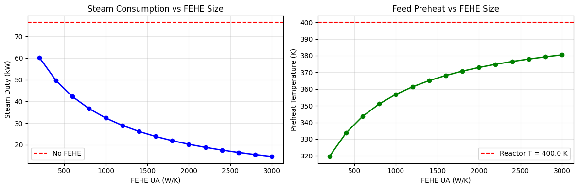
4.3 Effect of FEHE Size on Utility Consumption#
UA_range = jnp.linspace(200, 3000, 15)
steam_duties = []
preheat_temps = []

for UA in UA_range:
    result = process_with_heat_integration(float(UA))
    steam_duties.append(result['heater_duty'])
    preheat_temps.append(result['T_preheat'])

fig, axes = plt.subplots(1, 2, figsize=(12, 4))

# Base case steam duty
base_steam = float(heater_info['Q'])

axes[0].plot(UA_range, jnp.array(steam_duties)/1000, 'b-o', linewidth=2, markersize=6)
axes[0].axhline(y=base_steam/1000, color='r', linestyle='--', label='No FEHE')
axes[0].set_xlabel('FEHE UA (W/K)')
axes[0].set_ylabel('Steam Duty (kW)')
axes[0].set_title('Steam Consumption vs FEHE Size')
axes[0].legend()
axes[0].grid(True, alpha=0.3)

axes[1].plot(UA_range, preheat_temps, 'g-o', linewidth=2, markersize=6)
axes[1].axhline(y=T_reactor, color='r', linestyle='--', label=f'Reactor T = {T_reactor} K')
axes[1].set_xlabel('FEHE UA (W/K)')
axes[1].set_ylabel('Preheat Temperature (K)')
axes[1].set_title('Feed Preheat vs FEHE Size')
axes[1].legend()
axes[1].grid(True, alpha=0.3)

plt.tight_layout()
plt.show()
Summary#
This notebook demonstrated:
Heaters/Coolers: Single-stream heat exchange with utilities
Duty mode, temperature mode, and rating mode
Two-Stream Heat Exchangers:
Counter-current achieves highest effectiveness
Co-current is simpler but less efficient
Cross-flow offers intermediate performance with 4 mixing configurations:
Both unmixed (most common - car radiators, finned-tube HX)
Cmax mixed, Cmin mixed, both mixed
All fully differentiable using effectiveness-NTU method
Design Methods:
LMTD method when temperatures are known
Effectiveness-NTU method when flow rates are known
Heat Integration:
Feed-effluent heat exchanger (FEHE) reduces utility consumption
Trade-off between capital (larger HX) and operating (utility) costs
Optimization:
JAX gradients enable efficient optimization
Can minimize total annual cost (capital + operating)
Key Takeaway: Cross-flow heat exchangers provide a practical middle ground between counter-current (most efficient) and co-current (simplest), commonly used in applications like air-to-liquid heat transfer (HVAC, radiators).
def total_annual_cost(UA):
    """Calculate total annual cost as function of FEHE UA.

    TAC = Capital cost (annualized) + Operating cost (utilities)
    """
    # Capital cost: assume area = UA / U, with U = 500 W/m²·K
    U = 500.0  # W/m²·K
    A = UA / U  # m²

    # Equipment cost correlation: C = a * A^b
    # Typical for shell-and-tube: $1000/m² base
    equipment_cost = 5000.0 + 1000.0 * A  # $

    # Installed cost (Lang factor ~ 3)
    installed_cost = 3.0 * equipment_cost

    # Annualize over 10 years at 10% interest
    crf = 0.10 * (1.10**10) / ((1.10**10) - 1)  # Capital recovery factor
    annual_capital = installed_cost * crf

    # Operating cost: steam at $15/GJ, 8000 hours/year
    # Simulate to get steam duty
    cold_feed = make_stream({"A": 10.0, "B": 0.0}, T=298.0, P=101325.0)
    hot_product = make_stream({"A": 2.0, "B": 8.0}, T=400.0, P=101325.0)  # Approx reactor outlet

    # FEHE
    fehe = CounterCurrentHX(HeatExchangerParams(Cp_hot=77.5, Cp_cold=75.0))
    _, preheated, info = fehe(hot_product, cold_feed, UA=UA)

    # Trim heater duty
    T_preheat = preheated["T"]
    F_total = 10.0  # mol/s
    Cp = 75.0  # J/mol·K
    steam_duty = F_total * Cp * (400.0 - T_preheat)  # W

    # Annual steam cost
    steam_price = 15.0  # $/GJ
    hours_per_year = 8000.0
    annual_steam = steam_duty * hours_per_year * 3600 / 1e9 * steam_price  # $/year

    return annual_capital + annual_steam

# Evaluate TAC over range of UA (extended range to find true optimum)
UA_range = jnp.linspace(100, 5000, 50)
TAC_values = [float(total_annual_cost(jnp.array(ua))) for ua in UA_range]

# Find minimum
min_idx = jnp.argmin(jnp.array(TAC_values))
optimal_UA = float(UA_range[min_idx])
min_TAC = TAC_values[min_idx]

plt.figure(figsize=(10, 5))
plt.plot(UA_range, TAC_values, 'b-', linewidth=2, label='Total Annual Cost')
plt.axvline(x=optimal_UA, color='r', linestyle='--', label=f'Optimal UA = {optimal_UA:.0f} W/K')
plt.scatter([optimal_UA], [min_TAC], color='r', s=100, zorder=5)
plt.xlabel('FEHE UA (W/K)')
plt.ylabel('Total Annual Cost ($/year)')
plt.title('Heat Exchanger Optimization')
plt.legend()
plt.grid(True, alpha=0.3)
plt.show()

print(f"Optimal FEHE UA: {optimal_UA:.0f} W/K")
print(f"Optimal Area:    {optimal_UA/500:.2f} m²")
print(f"Minimum TAC:     ${min_TAC:,.0f}/year")
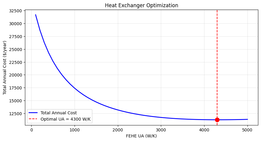
Optimal FEHE UA: 4300 W/K
Optimal Area:    8.60 m²
Minimum TAC:     $11,245/year
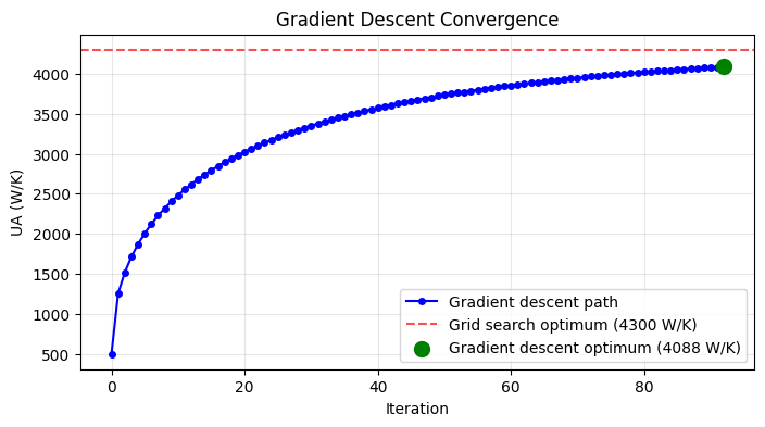
5.1 Gradient-Based Optimization#
# Use JAX gradients to optimize
grad_tac = jax.grad(total_annual_cost)

# Simple gradient descent
UA = jnp.array(500.0)  # Initial guess
learning_rate = 50.0
history = [float(UA)]

for i in range(500):
    g = grad_tac(UA)
    UA = UA - learning_rate * g
    UA = jnp.clip(UA, 100.0, 5000.0)  # Bounds
    history.append(float(UA))

    if abs(float(g)) < 0.1:
        break

final_UA = float(UA)
final_TAC = float(total_annual_cost(UA))

print(f"Gradient-based optimization:")
print(f"  Optimal UA:  {final_UA:.1f} W/K")
print(f"  Optimal TAC: ${final_TAC:,.0f}/year")
print(f"  Iterations:  {len(history)-1}")

# Compare with grid search
print(f"\nComparison:")
print(f"  Grid search:      {optimal_UA:.0f} W/K, TAC = ${min_TAC:,.0f}/year")
print(f"  Gradient descent: {final_UA:.0f} W/K, TAC = ${final_TAC:,.0f}/year")

# Plot convergence
plt.figure(figsize=(8, 4))
plt.plot(history, 'b-o', markersize=4, label='Gradient descent path')
plt.axhline(y=optimal_UA, color='r', linestyle='--', alpha=0.7, label=f'Grid search optimum ({optimal_UA:.0f} W/K)')
plt.scatter([len(history)-1], [final_UA], color='green', s=100, zorder=5,
            label=f'Gradient descent optimum ({final_UA:.0f} W/K)')
plt.xlabel('Iteration')
plt.ylabel('UA (W/K)')
plt.title('Gradient Descent Convergence')
plt.legend()
plt.grid(True, alpha=0.3)
plt.show()
Gradient-based optimization:
  Optimal UA:  4087.8 W/K
  Optimal TAC: $11,256/year
  Iterations:  92

Comparison:
  Grid search:      4300 W/K, TAC = $11,245/year
  Gradient descent: 4088 W/K, TAC = $11,256/year
Summary#
This notebook demonstrated:
Heaters/Coolers: Single-stream heat exchange with utilities
Duty mode, temperature mode, and rating mode
Two-Stream Heat Exchangers:
Counter-current achieves higher effectiveness
Both fully differentiable using effectiveness-NTU
Design Methods:
LMTD method when temperatures are known
Effectiveness-NTU method when flow rates are known
Heat Integration:
Feed-effluent heat exchanger (FEHE) reduces utility consumption
Trade-off between capital (larger HX) and operating (utility) costs
Optimization:
JAX gradients enable efficient optimization
Can minimize total annual cost (capital + operating)