
Differential Equations with JAX#
This notebook covers solving ordinary differential equations (ODEs) using JAX, with a focus on differentiable solvers that enable gradient-based optimization of dynamical systems.
Topics covered:
Basic ODE concepts and formulation
Simple Euler method implementation
Runge-Kutta methods (RK4)
Adaptive step size methods
Differentiating through ODE solutions
Parameter estimation in dynamical systems
Neural ODEs (introduction)
Using diffrax library
import jax
import jax.numpy as jnp
from jax import grad, jit, vmap, jacfwd
from jax import lax
import matplotlib.pyplot as plt
import numpy as np

# Enable 64-bit precision for better numerical accuracy
jax.config.update("jax_enable_x64", True)
1. ODE Basics#
An ordinary differential equation (ODE) describes how a quantity changes over time:
Given an initial condition \(y(t_0) = y_0\), we want to find \(y(t)\) for \(t > t_0\).
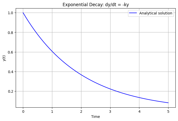
Example: Exponential Decay#
The simplest ODE is exponential decay: $\(\frac{dy}{dt} = -k \cdot y\)$
This has the analytical solution: \(y(t) = y_0 \cdot e^{-kt}\)
# Define the ODE right-hand side
def exponential_decay(t, y, k):
    """dy/dt = -k * y"""
    return -k * y

# Analytical solution for comparison
def analytical_solution(t, y0, k):
    return y0 * jnp.exp(-k * t)

# Test
k = 0.5
y0 = 1.0
t_test = jnp.linspace(0, 5, 50)
y_exact = analytical_solution(t_test, y0, k)

plt.figure(figsize=(8, 5))
plt.plot(t_test, y_exact, 'b-', label='Analytical solution')
plt.xlabel('Time')
plt.ylabel('y(t)')
plt.title('Exponential Decay: dy/dt = -ky')
plt.legend()
plt.grid(True)
plt.show()
WARNING:2026-01-10 20:25:59,656:jax._src.xla_bridge:852: An NVIDIA GPU may be present on this machine, but a CUDA-enabled jaxlib is not installed. Falling back to cpu.
2. Euler Method#
The simplest numerical method for solving ODEs is Euler’s method:
where \(h\) is the step size. This is a first-order method (error scales as \(O(h)\)).
Key insight for JAX:#
We use lax.scan to implement the time-stepping loop efficiently and differentiably.
def euler_step(f, t, y, h, *args):
    """Single Euler step."""
    return y + h * f(t, y, *args)

def euler_solve(f, y0, t_span, n_steps, *args):
    """
    Solve ODE using Euler method.

    Args:
        f: ODE function f(t, y, *args)
        y0: Initial condition
        t_span: (t_start, t_end)
        n_steps: Number of time steps
        *args: Additional arguments to f

    Returns:
        t_values: Time points
        y_values: Solution at each time point
    """
    t_start, t_end = t_span
    h = (t_end - t_start) / n_steps
    t_values = jnp.linspace(t_start, t_end, n_steps + 1)

    def scan_fn(y, t):
        y_new = euler_step(f, t, y, h, *args)
        return y_new, y_new

    # Use lax.scan for efficient, differentiable iteration
    _, y_values = lax.scan(scan_fn, y0, t_values[:-1])

    # Prepend initial condition
    y_values = jnp.concatenate([y0[None], y_values])

    return t_values, y_values

# Solve exponential decay with Euler method
t_euler, y_euler = euler_solve(exponential_decay, jnp.array([y0]), (0.0, 5.0), 50, k)

plt.figure(figsize=(8, 5))
plt.plot(t_test, y_exact, 'b-', label='Analytical', linewidth=2)
plt.plot(t_euler, y_euler[:, 0], 'r--', label='Euler (50 steps)', linewidth=2)
plt.xlabel('Time')
plt.ylabel('y(t)')
plt.title('Euler Method vs Analytical Solution')
plt.legend()
plt.grid(True)
plt.show()

# Check error
final_error = jnp.abs(y_euler[-1, 0] - analytical_solution(5.0, y0, k))
print(f"Final error with Euler: {final_error:.6f}")
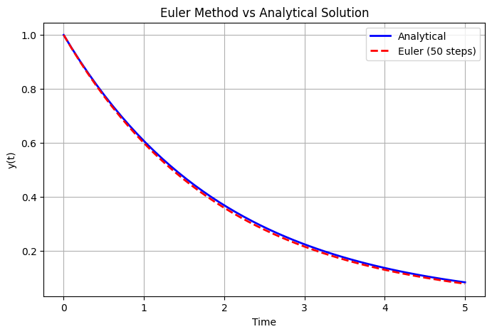
Final error with Euler: 0.005140
3. Runge-Kutta Methods (RK4)#
The 4th-order Runge-Kutta method is much more accurate (error \(O(h^4)\)):
def rk4_step(f, t, y, h, *args):
    """Single RK4 step."""
    k1 = f(t, y, *args)
    k2 = f(t + h/2, y + h*k1/2, *args)
    k3 = f(t + h/2, y + h*k2/2, *args)
    k4 = f(t + h, y + h*k3, *args)
    return y + (h/6) * (k1 + 2*k2 + 2*k3 + k4)

def rk4_solve(f, y0, t_span, n_steps, *args):
    """Solve ODE using RK4 method."""
    t_start, t_end = t_span
    h = (t_end - t_start) / n_steps
    t_values = jnp.linspace(t_start, t_end, n_steps + 1)

    def scan_fn(y, t):
        y_new = rk4_step(f, t, y, h, *args)
        return y_new, y_new

    _, y_values = lax.scan(scan_fn, y0, t_values[:-1])
    y_values = jnp.concatenate([y0[None], y_values])

    return t_values, y_values

# Compare Euler and RK4
t_rk4, y_rk4 = rk4_solve(exponential_decay, jnp.array([y0]), (0.0, 5.0), 50, k)

plt.figure(figsize=(10, 5))
plt.subplot(1, 2, 1)
plt.plot(t_test, y_exact, 'b-', label='Analytical', linewidth=2)
plt.plot(t_euler, y_euler[:, 0], 'r--', label='Euler', linewidth=2)
plt.plot(t_rk4, y_rk4[:, 0], 'g:', label='RK4', linewidth=2)
plt.xlabel('Time')
plt.ylabel('y(t)')
plt.title('Solution Comparison')
plt.legend()
plt.grid(True)

plt.subplot(1, 2, 2)
euler_errors = jnp.abs(y_euler[:, 0] - analytical_solution(t_euler, y0, k))
rk4_errors = jnp.abs(y_rk4[:, 0] - analytical_solution(t_rk4, y0, k))
plt.semilogy(t_euler, euler_errors, 'r-', label='Euler error')
plt.semilogy(t_rk4, rk4_errors, 'g-', label='RK4 error')
plt.xlabel('Time')
plt.ylabel('Absolute Error')
plt.title('Error Comparison (log scale)')
plt.legend()
plt.grid(True)
plt.tight_layout()
plt.show()

print(f"Final Euler error: {euler_errors[-1]:.2e}")
print(f"Final RK4 error: {rk4_errors[-1]:.2e}")
print(f"RK4 is {euler_errors[-1]/rk4_errors[-1]:.0f}x more accurate!")
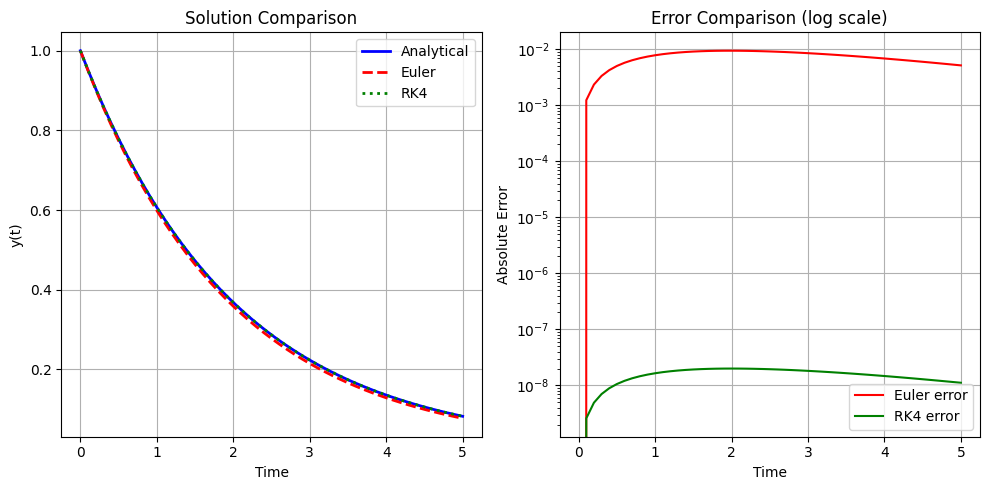
Final Euler error: 5.14e-03
Final RK4 error: 1.11e-08
RK4 is 461271x more accurate!
4. Systems of ODEs#
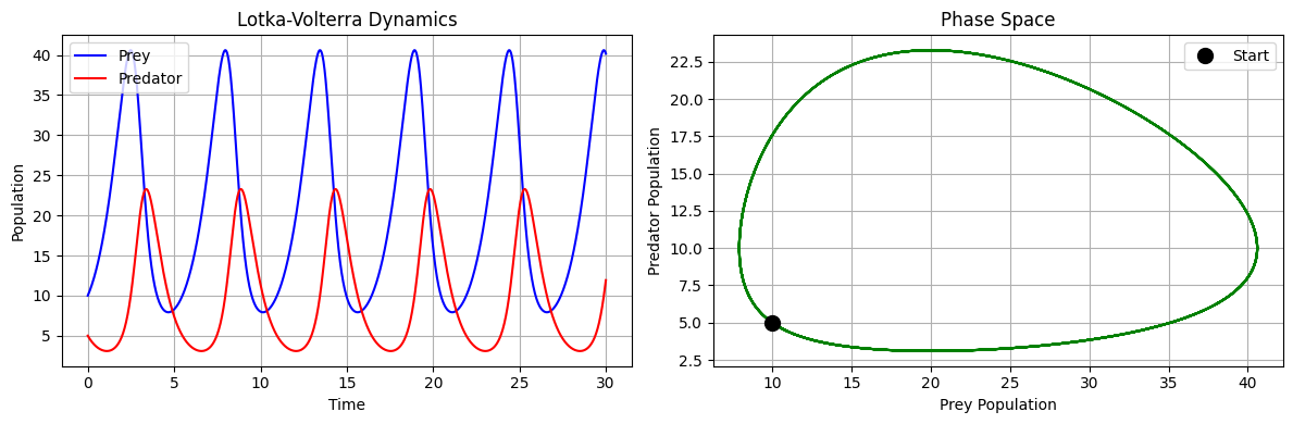
Real-world problems often involve systems of coupled ODEs. A classic example is the Lotka-Volterra predator-prey model:
where:
\(x\) = prey population
\(y\) = predator population
\(\alpha\) = prey growth rate
\(\beta\) = predation rate
\(\delta\) = predator growth from eating prey
\(\gamma\) = predator death rate
def lotka_volterra(t, state, params):
    """
    Lotka-Volterra predator-prey equations.

    state: [x, y] - prey and predator populations
    params: [alpha, beta, delta, gamma]
    """
    x, y = state
    alpha, beta, delta, gamma = params

    dx_dt = alpha * x - beta * x * y
    dy_dt = delta * x * y - gamma * y

    return jnp.array([dx_dt, dy_dt])

# Parameters
params = jnp.array([1.0, 0.1, 0.075, 1.5])  # alpha, beta, delta, gamma
y0_lv = jnp.array([10.0, 5.0])  # Initial populations

# Solve
t_lv, y_lv = rk4_solve(lotka_volterra, y0_lv, (0.0, 30.0), 1000, params)

plt.figure(figsize=(12, 4))

plt.subplot(1, 2, 1)
plt.plot(t_lv, y_lv[:, 0], 'b-', label='Prey')
plt.plot(t_lv, y_lv[:, 1], 'r-', label='Predator')
plt.xlabel('Time')
plt.ylabel('Population')
plt.title('Lotka-Volterra Dynamics')
plt.legend()
plt.grid(True)

plt.subplot(1, 2, 2)
plt.plot(y_lv[:, 0], y_lv[:, 1], 'g-')
plt.plot(y0_lv[0], y0_lv[1], 'ko', markersize=10, label='Start')
plt.xlabel('Prey Population')
plt.ylabel('Predator Population')
plt.title('Phase Space')
plt.legend()
plt.grid(True)

plt.tight_layout()
plt.show()
5. Differentiating Through ODE Solutions#
One of the most powerful features of JAX is the ability to differentiate through ODE solutions. This enables:
Parameter estimation from data
Optimal control
Sensitivity analysis
Neural ODEs
How it works:#
Because our ODE solver uses JAX primitives (lax.scan), gradients flow automatically through the entire integration!
# Let's compute the gradient of the final prey population w.r.t. parameters

def final_prey_population(params):
    """Returns final prey population given parameters."""
    _, y = rk4_solve(lotka_volterra, y0_lv, (0.0, 30.0), 500, params)
    return y[-1, 0]  # Final prey count

# Compute gradient
grad_params = grad(final_prey_population)(params)

print("Gradient of final prey population w.r.t. parameters:")
print(f"  d(prey)/d(alpha) = {grad_params[0]:.4f}  (prey growth rate)")
print(f"  d(prey)/d(beta)  = {grad_params[1]:.4f}  (predation rate)")
print(f"  d(prey)/d(delta) = {grad_params[2]:.4f}  (predator growth)")
print(f"  d(prey)/d(gamma) = {grad_params[3]:.4f}  (predator death rate)")
Gradient of final prey population w.r.t. parameters:
  d(prey)/d(alpha) = -94.5517  (prey growth rate)
  d(prey)/d(beta)  = -232.9485  (predation rate)
  d(prey)/d(delta) = -1207.4862  (predator growth)
  d(prey)/d(gamma) = -15.6146  (predator death rate)
# Verify gradient numerically
eps = 1e-5
numerical_grad = []
for i in range(4):
    params_plus = params.at[i].set(params[i] + eps)
    params_minus = params.at[i].set(params[i] - eps)
    numerical_grad.append(
        (final_prey_population(params_plus) - final_prey_population(params_minus)) / (2 * eps)
    )

print("\nNumerical vs Automatic Differentiation:")
for i, (name, num, auto) in enumerate(zip(
    ['alpha', 'beta', 'delta', 'gamma'],
    numerical_grad,
    grad_params
)):
    print(f"  {name}: numerical={num:.4f}, AD={auto:.4f}, diff={abs(num-auto):.2e}")
Numerical vs Automatic Differentiation:
  alpha: numerical=-94.5517, AD=-94.5517, diff=2.45e-06
  beta: numerical=-232.9485, AD=-232.9485, diff=2.11e-05
  delta: numerical=-1207.4858, AD=-1207.4862, diff=3.94e-04
  gamma: numerical=-15.6146, AD=-15.6146, diff=3.36e-07
6. Parameter Estimation#
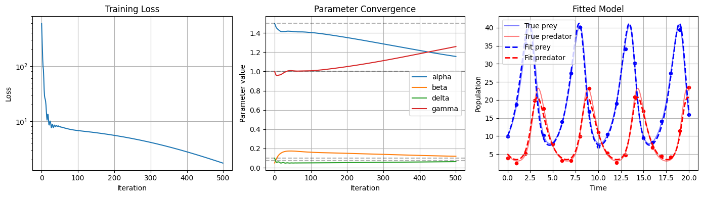
A common task is estimating ODE parameters from noisy data. We can use gradient-based optimization!
Problem Setup:#
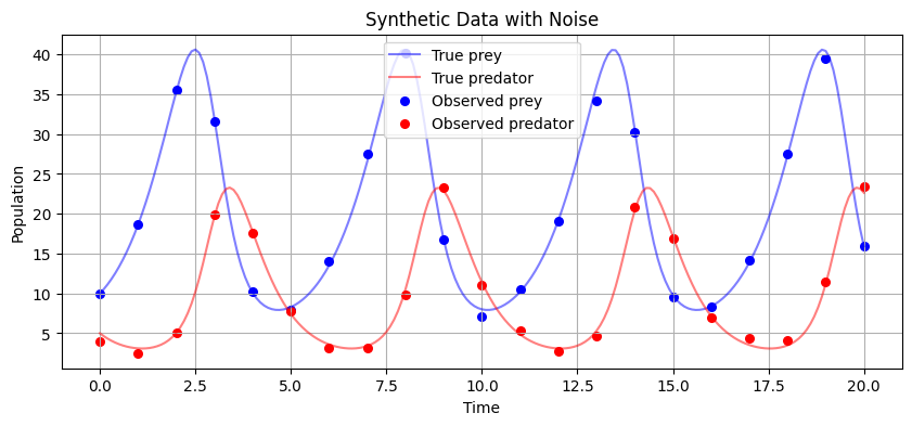
Generate “true” data with known parameters
Add noise
Estimate parameters by minimizing the difference between model predictions and data
# Generate "true" data
true_params = jnp.array([1.0, 0.1, 0.075, 1.5])
t_data, y_data = rk4_solve(lotka_volterra, y0_lv, (0.0, 20.0), 200, true_params)

# Add noise
key = jax.random.PRNGKey(42)
noise = jax.random.normal(key, y_data.shape) * 0.5
y_noisy = y_data + noise

# Subsample for "observations"
obs_indices = jnp.arange(0, 201, 10)  # Every 10th point
t_obs = t_data[obs_indices]
y_obs = y_noisy[obs_indices]

plt.figure(figsize=(10, 4))
plt.plot(t_data, y_data[:, 0], 'b-', alpha=0.5, label='True prey')
plt.plot(t_data, y_data[:, 1], 'r-', alpha=0.5, label='True predator')
plt.scatter(t_obs, y_obs[:, 0], c='b', s=30, label='Observed prey')
plt.scatter(t_obs, y_obs[:, 1], c='r', s=30, label='Observed predator')
plt.xlabel('Time')
plt.ylabel('Population')
plt.title('Synthetic Data with Noise')
plt.legend()
plt.grid(True)
plt.show()
def loss_function(params, t_obs, y_obs, y0):
    """
    Mean squared error between model predictions and observations.
    """
    # Solve ODE with current parameters
    t_full, y_full = rk4_solve(lotka_volterra, y0, (0.0, 20.0), 200, params)

    # Extract predictions at observation times
    y_pred = y_full[obs_indices]

    # MSE loss
    return jnp.mean((y_pred - y_obs) ** 2)

# JIT compile loss and gradient
loss_and_grad = jit(jax.value_and_grad(loss_function))

# Initial guess (wrong parameters)
params_init = jnp.array([1.5, 0.05, 0.1, 1.0])

# Adam optimizer (simple implementation)
def adam_update(params, grads, m, v, t, lr=0.01, beta1=0.9, beta2=0.999, eps=1e-8):
    m = beta1 * m + (1 - beta1) * grads
    v = beta2 * v + (1 - beta2) * grads**2
    m_hat = m / (1 - beta1**t)
    v_hat = v / (1 - beta2**t)
    params = params - lr * m_hat / (jnp.sqrt(v_hat) + eps)
    return params, m, v

# Run optimization
params = params_init
m = jnp.zeros_like(params)
v = jnp.zeros_like(params)

losses = []
param_history = [params]

for i in range(500):
    loss, grads = loss_and_grad(params, t_obs, y_obs, y0_lv)
    params, m, v = adam_update(params, grads, m, v, i + 1, lr=0.01)
    losses.append(loss)
    param_history.append(params)

    if i % 100 == 0:
        print(f"Iter {i:3d}: loss = {loss:.4f}, params = {params}")

print(f"\nFinal loss: {losses[-1]:.4f}")
print(f"Estimated params: {params}")
print(f"True params:      {true_params}")
Iter 0: loss = 597.3734, params = [1.49 0.06 0.09 0.99]
Iter 100: loss = 6.7464, params = [1.40414412 0.1610956 0.05109155 1.00733789]
Iter 200: loss = 5.5248, params = [1.35134688 0.14988996 0.05339044 1.05118675]
Iter 300: loss = 4.1141, params = [1.28519862 0.1388073 0.05647076 1.1130082 ]
Iter 400: loss = 2.7733, params = [1.21699062 0.12814908 0.06004305 1.18521159]
Final loss: 1.7321
Estimated params: [1.15577835 0.119258   0.06367057 1.25877098]
True params:      [1.    0.1   0.075 1.5  ]
# Visualize results
fig, axes = plt.subplots(1, 3, figsize=(14, 4))

# Loss curve
axes[0].semilogy(losses)
axes[0].set_xlabel('Iteration')
axes[0].set_ylabel('Loss')
axes[0].set_title('Training Loss')
axes[0].grid(True)

# Parameter convergence
param_history = jnp.array(param_history)
for i, name in enumerate(['alpha', 'beta', 'delta', 'gamma']):
    axes[1].plot(param_history[:, i], label=name)
    axes[1].axhline(y=true_params[i], color='k', linestyle='--', alpha=0.3)
axes[1].set_xlabel('Iteration')
axes[1].set_ylabel('Parameter value')
axes[1].set_title('Parameter Convergence')
axes[1].legend()
axes[1].grid(True)

# Final fit
_, y_fit = rk4_solve(lotka_volterra, y0_lv, (0.0, 20.0), 200, params)
axes[2].plot(t_data, y_data[:, 0], 'b-', alpha=0.5, label='True prey')
axes[2].plot(t_data, y_data[:, 1], 'r-', alpha=0.5, label='True predator')
axes[2].plot(t_data, y_fit[:, 0], 'b--', linewidth=2, label='Fit prey')
axes[2].plot(t_data, y_fit[:, 1], 'r--', linewidth=2, label='Fit predator')
axes[2].scatter(t_obs, y_obs[:, 0], c='b', s=20)
axes[2].scatter(t_obs, y_obs[:, 1], c='r', s=20)
axes[2].set_xlabel('Time')
axes[2].set_ylabel('Population')
axes[2].set_title('Fitted Model')
axes[2].legend()
axes[2].grid(True)

plt.tight_layout()
plt.show()
7. Stiff ODEs and Chemical Kinetics#
Stiff ODEs have widely varying time scales, making them challenging to solve with explicit methods like RK4.
A classic example is the Robertson chemical kinetics problem:
The rate constants span 11 orders of magnitude!
def robertson(t, y, params):
    """Robertson chemical kinetics (stiff ODE)."""
    k1, k2, k3 = params
    y1, y2, y3 = y

    dy1 = -k1 * y1 + k2 * y2 * y3
    dy2 = k1 * y1 - k2 * y2 * y3 - k3 * y2**2
    dy3 = k3 * y2**2

    return jnp.array([dy1, dy2, dy3])

params_rob = jnp.array([0.04, 1e4, 3e7])
y0_rob = jnp.array([1.0, 0.0, 0.0])

# Solve with many steps (needed for stiff problems with explicit methods)
t_rob, y_rob = rk4_solve(robertson, y0_rob, (0.0, 40.0), 100000, params_rob)

plt.figure(figsize=(10, 4))
plt.subplot(1, 2, 1)
plt.plot(t_rob, y_rob[:, 0], label='y1')
plt.plot(t_rob, y_rob[:, 2], label='y3')
plt.xlabel('Time')
plt.ylabel('Concentration')
plt.title('Robertson Problem (y1, y3)')
plt.legend()
plt.grid(True)

plt.subplot(1, 2, 2)
plt.semilogy(t_rob, y_rob[:, 1] * 1e4, label='y2 × 10⁴')
plt.xlabel('Time')
plt.ylabel('Concentration')
plt.title('Robertson Problem (y2, scaled)')
plt.legend()
plt.grid(True)

plt.tight_layout()
plt.show()

print(f"Mass conservation: {y_rob[-1].sum():.10f} (should be 1.0)")
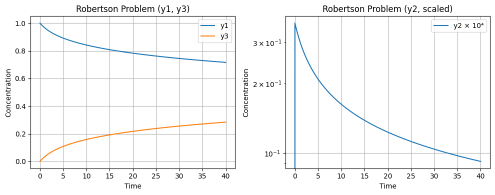
Mass conservation: 1.0000000000 (should be 1.0)
8. Implicit Methods for Stiff ODEs#
For stiff problems, implicit methods are more stable. The simplest is the Backward Euler method:
This requires solving a nonlinear equation at each step. We can use Newton’s method.
def backward_euler_step(f, t_new, y_old, h, args, max_iter=10, tol=1e-10):
    """
    Backward Euler step using Newton iteration.

    Solves: y_new = y_old + h * f(t_new, y_new)
    Rearranged: g(y) = y - y_old - h * f(t_new, y) = 0
    """
    def residual(y):
        return y - y_old - h * f(t_new, y, *args)

    # Initial guess from forward Euler
    y = y_old + h * f(t_new - h, y_old, *args)

    # Newton iteration
    def newton_step(carry, _):
        y, converged = carry
        r = residual(y)
        J = jacfwd(residual)(y)

        # Solve J @ dy = -r
        dy = jnp.linalg.solve(J, -r)
        y_new = y + dy

        # Check convergence
        converged = jnp.linalg.norm(dy) < tol

        return (y_new, converged), None

    (y_final, _), _ = lax.scan(newton_step, (y, False), None, length=max_iter)
    return y_final

def backward_euler_solve(f, y0, t_span, n_steps, *args):
    """Solve ODE using Backward Euler method."""
    t_start, t_end = t_span
    h = (t_end - t_start) / n_steps
    t_values = jnp.linspace(t_start, t_end, n_steps + 1)

    def scan_fn(y, t_new):
        y_new = backward_euler_step(f, t_new, y, h, args)
        return y_new, y_new

    _, y_values = lax.scan(scan_fn, y0, t_values[1:])
    y_values = jnp.concatenate([y0[None], y_values])

    return t_values, y_values

# Solve Robertson problem with backward Euler (fewer steps needed!)
t_be, y_be = backward_euler_solve(robertson, y0_rob, (0.0, 40.0), 1000, params_rob)

plt.figure(figsize=(10, 4))
plt.subplot(1, 2, 1)
plt.plot(t_be, y_be[:, 0], label='y1 (BE)')
plt.plot(t_be, y_be[:, 2], label='y3 (BE)')
plt.xlabel('Time')
plt.ylabel('Concentration')
plt.title('Backward Euler (1000 steps)')
plt.legend()
plt.grid(True)

plt.subplot(1, 2, 2)
plt.semilogy(t_be, y_be[:, 1] * 1e4, label='y2 × 10⁴ (BE)')
plt.xlabel('Time')
plt.ylabel('Concentration')
plt.title('Backward Euler (y2, scaled)')
plt.legend()
plt.grid(True)

plt.tight_layout()
plt.show()

print(f"Mass conservation: {y_be[-1].sum():.10f} (should be 1.0)")
print(f"\nComparison: RK4 needed 100,000 steps, Backward Euler only 1,000!")
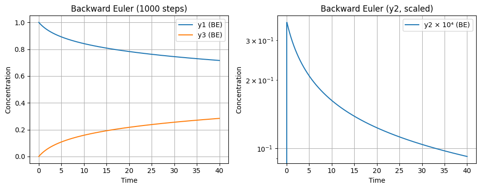
Mass conservation: 1.0000000000 (should be 1.0)

Comparison: RK4 needed 100,000 steps, Backward Euler only 1,000!
9. Sensitivity Analysis of ODEs#
The sensitivity \(s_i = \frac{\partial y}{\partial p_i}\) tells us how the solution changes with respect to parameters.
There are two approaches:
9.1 Forward Sensitivity (solve augmented system)#
Differentiate the ODE \(\frac{dy}{dt} = f(t, y, p)\) w.r.t. \(p\):
def forward_sensitivity_system(t, augmented_state, params):
    """
    Augmented system for forward sensitivity analysis.

    augmented_state contains:
    - y: the state (first n_y elements)
    - S: the sensitivity matrix dy/dp (flattened, remaining elements)
    """
    n_y = 2  # Number of state variables (Lotka-Volterra)
    n_p = 4  # Number of parameters

    y = augmented_state[:n_y]
    S = augmented_state[n_y:].reshape(n_y, n_p)

    # Original ODE
    f = lotka_volterra(t, y, params)

    # Jacobians
    df_dy = jacfwd(lambda y_: lotka_volterra(t, y_, params))(y)
    df_dp = jacfwd(lambda p: lotka_volterra(t, y, p))(params)

    # Sensitivity ODE: dS/dt = df/dy @ S + df/dp
    dS_dt = df_dy @ S + df_dp

    return jnp.concatenate([f, dS_dt.flatten()])

# Initial conditions: y0, and zero sensitivities
S0 = jnp.zeros((2, 4))  # Initial sensitivity is zero
augmented_y0 = jnp.concatenate([y0_lv, S0.flatten()])

# Solve
t_sens, y_sens = rk4_solve(forward_sensitivity_system, augmented_y0, (0.0, 20.0), 500, true_params)

# Extract sensitivity
y_solution = y_sens[:, :2]
S_final = y_sens[-1, 2:].reshape(2, 4)

print("Forward sensitivity at t=20:")
print("\ndx/dp (prey sensitivity to parameters):")
for i, name in enumerate(['alpha', 'beta', 'delta', 'gamma']):
    print(f"  d(prey)/d({name}) = {S_final[0, i]:+.4f}")

print("\ndy/dp (predator sensitivity to parameters):")
for i, name in enumerate(['alpha', 'beta', 'delta', 'gamma']):
    print(f"  d(pred)/d({name}) = {S_final[1, i]:+.4f}")
Forward sensitivity at t=20:

dx/dp (prey sensitivity to parameters):
  d(prey)/d(alpha) = -208.6077
  d(prey)/d(beta) = -72.6854
  d(prey)/d(delta) = -893.1252
  d(prey)/d(gamma) = -79.2722

dy/dp (predator sensitivity to parameters):
  d(pred)/d(alpha) = -45.1292
  d(pred)/d(beta) = -341.0425
  d(pred)/d(delta) = -414.8330
  d(pred)/d(gamma) = -19.1154
9.2 Adjoint Sensitivity (more efficient for many parameters)#
JAX’s reverse-mode autodiff automatically implements adjoint sensitivity when you differentiate through lax.scan. This is more efficient when you have many parameters but few outputs.
# Using JAX's automatic adjoint through lax.scan
def final_state_loss(params):
    """Sum of final populations."""
    _, y = rk4_solve(lotka_volterra, y0_lv, (0.0, 20.0), 500, params)
    return y[-1, 0] + y[-1, 1]

# This uses adjoint method automatically!
adjoint_grad = grad(final_state_loss)(true_params)

print("Adjoint sensitivity (d(prey + pred)/dp at t=20):")
for i, name in enumerate(['alpha', 'beta', 'delta', 'gamma']):
    forward_sens = S_final[0, i] + S_final[1, i]  # Sum of sensitivities
    print(f"  d(sum)/d({name}): adjoint = {adjoint_grad[i]:+.4f}, forward = {forward_sens:+.4f}")
Adjoint sensitivity (d(prey + pred)/dp at t=20):
  d(sum)/d(alpha): adjoint = -253.7370, forward = -253.7370
  d(sum)/d(beta): adjoint = -413.7279, forward = -413.7279
  d(sum)/d(delta): adjoint = -1307.9583, forward = -1307.9583
  d(sum)/d(gamma): adjoint = -98.3877, forward = -98.3877
10. Using diffrax Library#
For production use, the diffrax library provides high-quality, differentiable ODE solvers with:
Adaptive step size control
Multiple solver types (Dopri5, Tsit5, implicit methods)
Event handling
Efficient adjoints
# Install with: pip install diffrax
import diffrax

def vector_field(t, y, args):
    return lotka_volterra(t, y, args)

term = diffrax.ODETerm(vector_field)
solver = diffrax.Dopri5()
solution = diffrax.diffeqsolve(
    term,
    solver,
    t0=0,
    t1=20,
    dt0=0.1,
    y0=y0_lv,
    args=true_params,
    saveat=diffrax.SaveAt(ts=jnp.linspace(0, 20, 100))
)
11. Neural ODEs (Introduction)#
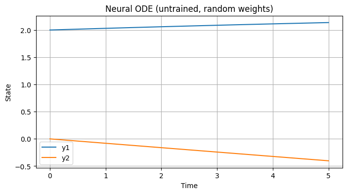
Neural ODEs replace the right-hand side \(f(t, y)\) with a neural network:
This creates a continuous-depth neural network that can be trained end-to-end through the ODE solver.
def neural_ode_field(t, y, params):
    """
    Simple neural network for ODE right-hand side.

    params: dict with 'W1', 'b1', 'W2', 'b2'
    """
    W1, b1, W2, b2 = params['W1'], params['b1'], params['W2'], params['b2']

    # Simple 2-layer MLP
    h = jnp.tanh(W1 @ y + b1)
    return W2 @ h + b2

def init_neural_ode_params(key, input_dim, hidden_dim):
    """Initialize neural ODE parameters."""
    keys = jax.random.split(key, 4)
    scale = 0.1
    return {
        'W1': jax.random.normal(keys[0], (hidden_dim, input_dim)) * scale,
        'b1': jnp.zeros(hidden_dim),
        'W2': jax.random.normal(keys[2], (input_dim, hidden_dim)) * scale,
        'b2': jnp.zeros(input_dim),
    }

# Initialize
key = jax.random.PRNGKey(0)
node_params = init_neural_ode_params(key, input_dim=2, hidden_dim=32)

# Solve neural ODE
def solve_neural_ode(params, y0, t_span, n_steps):
    t_start, t_end = t_span
    h = (t_end - t_start) / n_steps
    t_values = jnp.linspace(t_start, t_end, n_steps + 1)

    def scan_fn(y, t):
        # RK4 step
        k1 = neural_ode_field(t, y, params)
        k2 = neural_ode_field(t + h/2, y + h*k1/2, params)
        k3 = neural_ode_field(t + h/2, y + h*k2/2, params)
        k4 = neural_ode_field(t + h, y + h*k3, params)
        y_new = y + (h/6) * (k1 + 2*k2 + 2*k3 + k4)
        return y_new, y_new

    _, y_values = lax.scan(scan_fn, y0, t_values[:-1])
    y_values = jnp.concatenate([y0[None], y_values])

    return t_values, y_values

# Test forward pass
y0_node = jnp.array([2.0, 0.0])
t_node, y_node = solve_neural_ode(node_params, y0_node, (0.0, 5.0), 100)

plt.figure(figsize=(8, 4))
plt.plot(t_node, y_node[:, 0], label='y1')
plt.plot(t_node, y_node[:, 1], label='y2')
plt.xlabel('Time')
plt.ylabel('State')
plt.title('Neural ODE (untrained, random weights)')
plt.legend()
plt.grid(True)
plt.show()
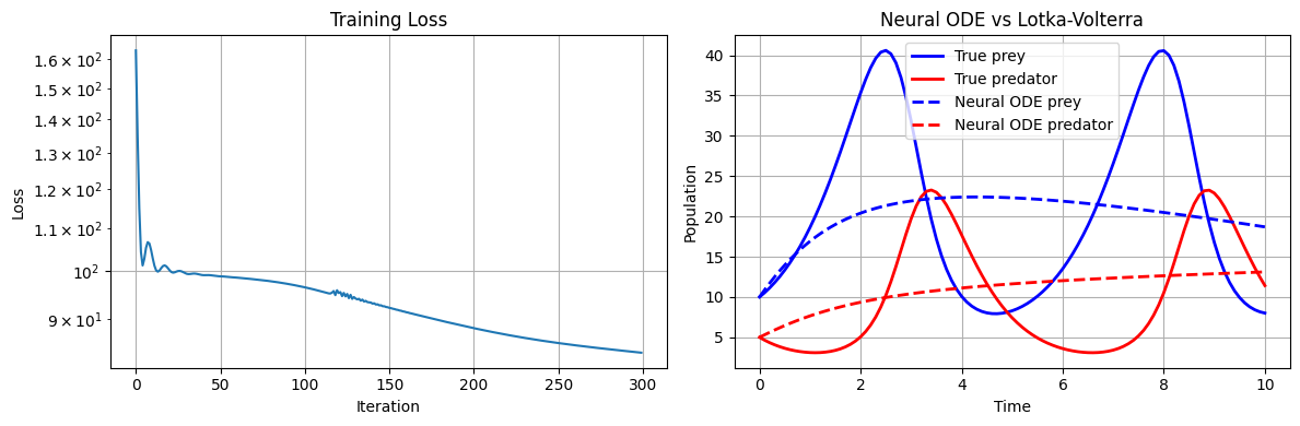
# Train neural ODE to mimic Lotka-Volterra
# Generate training data
t_train, y_train = rk4_solve(lotka_volterra, y0_lv, (0.0, 10.0), 100, true_params)

def node_loss(params, t_data, y_data):
    """MSE loss for neural ODE."""
    _, y_pred = solve_neural_ode(params, y_data[0], (t_data[0], t_data[-1]), len(t_data) - 1)
    return jnp.mean((y_pred - y_data) ** 2)

# Training loop
node_loss_and_grad = jit(jax.value_and_grad(node_loss))

# Initialize optimizer state for each parameter
m = jax.tree.map(jnp.zeros_like, node_params)
v = jax.tree.map(jnp.zeros_like, node_params)

def adam_update_tree(params, grads, m, v, t, lr=0.01):
    beta1, beta2, eps = 0.9, 0.999, 1e-8
    m = jax.tree.map(lambda m_, g: beta1 * m_ + (1 - beta1) * g, m, grads)
    v = jax.tree.map(lambda v_, g: beta2 * v_ + (1 - beta2) * g**2, v, grads)
    m_hat = jax.tree.map(lambda m_: m_ / (1 - beta1**t), m)
    v_hat = jax.tree.map(lambda v_: v_ / (1 - beta2**t), v)
    params = jax.tree.map(
        lambda p, m_, v_: p - lr * m_ / (jnp.sqrt(v_) + eps),
        params, m_hat, v_hat
    )
    return params, m, v

losses = []
for i in range(300):
    loss, grads = node_loss_and_grad(node_params, t_train, y_train)
    node_params, m, v = adam_update_tree(node_params, grads, m, v, i + 1, lr=0.01)
    losses.append(loss)

    if i % 50 == 0:
        print(f"Iter {i}: loss = {loss:.6f}")

print(f"\nFinal loss: {losses[-1]:.6f}")
Iter 0: loss = 163.206654
Iter 50: loss = 98.864786
Iter 100: loss = 96.473752
Iter 150: loss = 92.174207
Iter 200: loss = 88.112829
Iter 250: loss = 85.252522

Final loss: 83.448991
# Visualize trained neural ODE
_, y_node_trained = solve_neural_ode(node_params, y0_lv, (0.0, 10.0), 100)

fig, axes = plt.subplots(1, 2, figsize=(12, 4))

axes[0].semilogy(losses)
axes[0].set_xlabel('Iteration')
axes[0].set_ylabel('Loss')
axes[0].set_title('Training Loss')
axes[0].grid(True)

axes[1].plot(t_train, y_train[:, 0], 'b-', label='True prey', linewidth=2)
axes[1].plot(t_train, y_train[:, 1], 'r-', label='True predator', linewidth=2)
axes[1].plot(t_train, y_node_trained[:, 0], 'b--', label='Neural ODE prey', linewidth=2)
axes[1].plot(t_train, y_node_trained[:, 1], 'r--', label='Neural ODE predator', linewidth=2)
axes[1].set_xlabel('Time')
axes[1].set_ylabel('Population')
axes[1].set_title('Neural ODE vs Lotka-Volterra')
axes[1].legend()
axes[1].grid(True)

plt.tight_layout()
plt.show()
Summary#
In this notebook, we covered:
Basic ODE solvers - Euler and RK4 methods using
lax.scanSystems of ODEs - Lotka-Volterra predator-prey model
Differentiating through solutions - JAX handles this automatically
Parameter estimation - Fitting ODE parameters to data
Stiff ODEs - Implicit methods for challenging problems
Sensitivity analysis - Forward and adjoint methods
Neural ODEs - Neural networks as ODE right-hand sides
Key takeaways:#
lax.scanis perfect for time-stepping algorithms - efficient and differentiableJAX’s autodiff flows through the entire ODE solver automatically
Implicit methods need Newton iteration but handle stiff problems better
For production use, consider diffrax for adaptive step size and efficient adjoints
Neural ODEs combine deep learning with dynamical systems