Stochastic Programming: Nd/Dy Separation with Uncertain Distribution Coefficients

Stochastic Programming: Nd/Dy Separation with Uncertain Distribution Coefficients#

Every number in a solvent-extraction design rests on a distribution coefficient, and every distribution coefficient is a regression output with a standard error. The correlations in difflow_ree’s extractant database are of the form

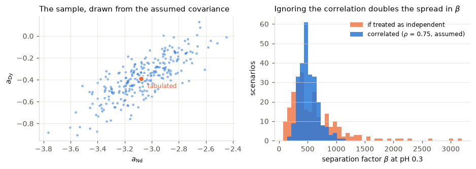
\[\log_{10} D_i = a_i + b_i\,\mathrm{pH} + c_i\,\mathrm{pH}^2 + \dots\]

and $a_i$ is $\log_{10} D_i$ at the reference condition. A perfectly ordinary fitting uncertainty of $0.2$ in $a$ is therefore a factor of $1.6$ in $D$ — and what a separation plant actually lives or dies on is the ratio of two $D$’s, the separation factor $\beta = D_{\mathrm{Dy}}/D_{\mathrm{Nd}}$.

This notebook designs a Nd/Dy extraction section that has to work anyway. It uses difflow.stochastic, which turns the design into a two-stage stochastic program and solves its sample average approximation with the same JAX gradients everything else in difflow runs on.

The four questions it answers, in order:

What does the coefficient uncertainty do to the separation?
What happens if you design at the nominal coefficients and hope?
What design should you build instead, and what is that worth? (VSS)
Should you go and measure the coefficients instead? (EVPI)

The fourth answer turns out to be the interesting one.

Before any number in here is copied#

This notebook is a demonstration of difflow.stochastic, and four of its inputs are not measurements:

SIGMA is a hypothesis, not this record’s fit. PC88A’s intercepts are MEASURED — refit in #270 against Tanaka et al. (2021), one free parameter per element over 121 digitized points, with the slope pinned at the proton stoichiometry b = 3. The standard errors that fit returned are 0.033 for Nd and 0.021 for Dy, six to nine times tighter than the 0.20 / 0.18 used below. Read SIGMA as “what if the coefficients were only as good as a typical literature correlation” — which is the interesting case, and the case most extractant data is actually in — rather than as a property of this record. Run it again with 0.033/0.021 and every gap in section 6 shrinks toward zero, which is the point: good data is worth what the stochastic program says it is worth.
RHO = 0.75 is assumed, not fitted. PC88A’s refit fits each element’s intercept on its own pH series, so the two estimates are essentially uncorrelated: the fit implies RHO near 0, not 0.75. This one matters more than the others. Section 6 reruns the bounds at RHO = 0: the VSS goes from $3.9M to about $38M/yr.
The operating pH lands near 0.4, low in the fitted window. PC88A’s declared window is (0.1, 2.5), so nothing here extrapolates the record. It does sit below the pH range Tanaka’s Nd series covers (0.68–2.37; the Dy series runs 0.12–1.24), so the Nd line down there is the pinned b = 3 mass action rather than a measured point. That is the one place a real study would want a confirming datum.
The Dy price is ESTIMATED, not sourced. $450/kg Dy₂O₃ carries the tag EST; only La, Ce, Pr, Nd, Eu and Gd were updated to USGS 2025 averages. Every dollar figure downstream — the $3.9M VSS, the $74M that the pH loop is worth — scales with it roughly linearly.
CLEANUP, SOLVENT_COST and STAGE_COST are illustrative. They set the shape of the trade-off, not its magnitude.

What the notebook is really demonstrating is the structure of the answer — a small VSS and an EVPI of essentially zero while a pH loop is free to move, and a mean-value design that is not even admissible once that loop is taken away — and that structure survives a factor of two in the price or the costs, and a SIGMA six to nine times tighter. The small VSS does not survive dropping the assumed correlation (section 6); the near-zero EVPI does.

1. Setup#

A heavy-REE chloride liquor: mostly Nd, with the Dy that pays for the plant. PC88A extracts the heavier lanthanide preferentially — $\beta_{\rm Dy/Nd}$ is about 490 on this record — so a single counter-current section can concentrate Dy, if the pH is right. PC88A rather than D2EHPA because this is the cut PC88A is actually run for: since the #270 refit D2EHPA’s fitted window is $[0, 2]$ and it extracts Nd quantitatively across nearly all of it, which leaves no interior operating point for a Nd/Dy section to trade off.

import time

import jax
import jax.numpy as jnp
import numpy as np

jax.config.update("jax_enable_x64", True)

import difflow.stochastic as st
from difflow import get_flows, make_stream
from difflow_ree import REEExtractor, REEExtractorParams, get_element
from difflow_ree.equilibrium.distribution import REEDistribution
from difflow_ree.provenance import explain

ELEMENTS = ("Nd", "Dy")
FEED = {"Nd": 1.00, "Dy": 0.12}      # mol/s
WATER = 55.0                          # mol/s of aqueous carrier
HOURS = 8000.0 * 3600.0               # operating seconds per year

# Prices in this database are OXIDE prices -- $/kg of RE2O3, which is how the
# USGS quotes them and how the trade is done. They are NOT $/kg of metal. A mole
# of Dy in the extract is half a mole of Dy2O3 on the invoice, so the mass that
# gets priced is oxide_mw/2, not atomic_weight. Pricing the metal mass at the
# oxide price undervalues Dy by 15% and Nd by 17%, straight off the top line.
for _e in ELEMENTS:
    assert get_element(_e).oxide_formula == f"{_e}2O3"
OXIDE_KG_PER_MOL = {e: get_element(e).oxide_mw / 2.0 * 1e-3 for e in ELEMENTS}
PRICE = {e: get_element(e).price_usd_kg for e in ELEMENTS}   # $/kg of RE2O3

# Economics, all annualised.
CLEANUP = 250.0        # $/kg of Nd2O3 the downstream train has to take back out
SOLVENT_COST = 5.0e5   # $/yr per mol/s of organic circulated
STAGE_COST = 8.0e6     # $/yr per equilibrium stage, annualised capital

nominal = REEDistribution(extractant="PC88A", elements=ELEMENTS)
A_NOM = np.array([float(nominal._coefficients(e).a) for e in ELEMENTS])

print("tabulated log10(D) intercepts:",
      {e: round(float(a), 3) for e, a in zip(ELEMENTS, A_NOM)},
      " provenance:",
      {e: explain("extractants", f"extractants.PC88A.ph_coefficients.{e}.a").cls
       for e in ELEMENTS})
for e in ELEMENTS:
    p = explain("elements", f"elements.{e}.price_usd_kg")
    print(f"  {e}: ${PRICE[e]:>7.2f}/kg {e}2O3  "
          f"({OXIDE_KG_PER_MOL[e] * 1e3:.1f} g of oxide per mol of metal)"
          f"   [{p.cls} / {p.source}]")
print()
print(f"{'pH':>5}{'D_Nd':>10}{'D_Dy':>12}{'beta':>8}")
for pH in (0.2, 0.3, 0.4, 0.5):
    D = {e: float(nominal.get_D(e, pH=pH)) for e in ELEMENTS}
    print(f"{pH:5.1f}{D['Nd']:10.4f}{D['Dy']:12.4f}{D['Dy'] / D['Nd']:8.0f}")

tabulated log10(D) intercepts: {'Nd': -3.078, 'Dy': -0.391}  provenance: {'Nd': 'MEASURED', 'Dy': 'MEASURED'}
  Nd: $  69.00/kg Nd2O3  (168.2 g of oxide per mol of metal)   [REFERENCE / USGS26]
  Dy: $ 450.00/kg Dy2O3  (186.5 g of oxide per mol of metal)   [ESTIMATED / EST]

   pH      D_Nd        D_Dy    beta
  0.2    0.0033      1.6199     487
  0.3    0.0066      3.2322     487
  0.4    0.0133      6.4491     487
  0.5    0.0264     12.8677     487

That table is the whole engineering problem in four rows, and note what is not in it: $\beta$ does not move. Every element on this record shares the stoichiometric slope $b = 3$, so $\beta = 10^{a_{\mathrm{Dy}} - a_{\mathrm{Nd}}}$ is one number at every pH — that is what #265 and #270 fixed. What pH does move is level: it raises $D_{\mathrm{Dy}}$, which buys Dy recovery, and it raises $D_{\mathrm{Nd}}$ by exactly the same factor of a thousand per pH unit, which costs Dy purity and loads the extractant closer to saturation. Recovery against purity is the interior trade-off, and where it sits depends on coefficients nobody knows exactly.

Figures#

The plotting helpers, kept out of the way. One fixed categorical order, checked colourblind-safe; nothing below depends on them.

import matplotlib.pyplot as plt
import numpy as np

# One categorical order, fixed, validated colorblind-safe (deutan dE 9.2,
# tritan 32.7, normal 27.6 -- scripts/validate_palette.js).
BLUE, ORANGE, AQUA = "#2a78d6", "#eb6834", "#1baf7a"
INK, MUTED, GRID = "#0b0b0b", "#52514e", "#dcdbd6"

plt.rcParams.update({
    "figure.dpi": 110, "savefig.dpi": 110,
    "font.size": 9, "axes.titlesize": 10, "axes.labelsize": 9,
    "axes.edgecolor": GRID, "axes.labelcolor": INK,
    "axes.spines.top": False, "axes.spines.right": False,
    "xtick.color": MUTED, "ytick.color": MUTED,
    "grid.color": GRID, "grid.linewidth": 0.6,
    "legend.frameon": False, "figure.facecolor": "white",
})


def fig_uncertainty(scenarios, independent, A_NOM, nominal, ELEMENTS,
                    pH=0.3):
    """What the coefficient uncertainty does to the separation factor."""
    b = nominal._coefficients
    slope = {e: float(b(e).b) for e in ELEMENTS}
    curv = {e: float(b(e).c) for e in ELEMENTS}

    def beta_of(sample):
        d = np.asarray(sample.draws)
        logD = {e: d[:, i] + slope[e] * pH + curv[e] * pH ** 2
                for i, e in enumerate(ELEMENTS)}
        return 10.0 ** (logD["Dy"] - logD["Nd"])

    d = np.asarray(scenarios.draws)
    beta, beta_indep = beta_of(scenarios), beta_of(independent)

    fig, ax = plt.subplots(1, 2, figsize=(8.6, 3.1))
    ax[0].scatter(d[:, 0], d[:, 1], s=9, color=BLUE, alpha=0.55,
                  linewidths=0)
    ax[0].scatter([A_NOM[0]], [A_NOM[1]], s=46, color=ORANGE, zorder=3,
                  edgecolor="white", linewidth=1.2)
    ax[0].annotate("tabulated", (A_NOM[0], A_NOM[1]),
                   textcoords="offset points", xytext=(8, -12),
                   color=ORANGE, fontsize=8)
    ax[0].set_xlabel(r"$a_{\mathrm{Nd}}$")
    ax[0].set_ylabel(r"$a_{\mathrm{Dy}}$")
    ax[0].set_title("The sample, drawn from the assumed covariance", loc="left")
    ax[0].grid(True, linewidth=0.6, alpha=0.7)

    bins = np.linspace(min(beta.min(), beta_indep.min()),
                       max(beta.max(), beta_indep.max()), 44)
    ax[1].hist(beta_indep, bins=bins, color=ORANGE, alpha=0.75,
               label="if treated as independent")
    ax[1].hist(beta, bins=bins, color=BLUE, alpha=0.85,
               label=r"correlated ($\rho$ = 0.75, assumed)")
    ax[1].set_xlabel(rf"separation factor $\beta$ at pH {pH}")
    ax[1].set_ylabel("scenarios")
    ax[1].set_title(r"Ignoring the correlation doubles the spread in $\beta$",
                    loc="left")
    ax[1].legend(loc="upper right", fontsize=8)
    ax[1].grid(True, axis="y", linewidth=0.6, alpha=0.7)
    fig.tight_layout()
    return fig


def fig_designs(det, sto, spec):
    """Two designs, two profit distributions, one specification."""
    fig, ax = plt.subplots(1, 2, figsize=(8.6, 3.1))
    lo = min(det.objective_values.min(), sto.objective_values.min())
    hi = max(det.objective_values.max(), sto.objective_values.max())
    bins = np.linspace(lo, hi, 46)
    ax[0].hist(det.objective_values, bins=bins, color=ORANGE, alpha=0.8,
               label="mean-value design")
    ax[0].hist(sto.objective_values, bins=bins, color=BLUE, alpha=0.85,
               label="stochastic design")
    for r, c in ((det, ORANGE), (sto, BLUE)):
        ax[0].axvline(r.risk_value, color=c, linewidth=2.0, linestyle="--")
    ax[0].set_xlabel("profit  ($M/yr)")
    ax[0].set_ylabel("scenarios")
    ax[0].set_title("Dashed line: the CVaR each design was scored on",
                    loc="left")
    ax[0].legend(loc="upper left", fontsize=8)
    ax[0].grid(True, axis="y", linewidth=0.6, alpha=0.7)

    pd_, ps = det.outputs["purity"], sto.outputs["purity"]
    bins = np.linspace(min(pd_.min(), ps.min()), max(pd_.max(), ps.max()), 46)
    ax[1].hist(pd_, bins=bins, color=ORANGE, alpha=0.8,
               label=f"mean-value ({det.violation_rates[0]:.0%} off spec)")
    ax[1].hist(ps, bins=bins, color=BLUE, alpha=0.85,
               label=f"stochastic ({sto.violation_rates[0]:.0%} off spec)")
    ax[1].axvline(spec, color=INK, linewidth=1.4)
    ax[1].annotate(f"spec {spec:g}", (spec, ax[1].get_ylim()[1] * 0.06),
                   textcoords="offset points", xytext=(5, 0), fontsize=8,
                   color=INK)
    ax[1].set_xlabel("Dy purity in the extract  (mol/mol)")
    ax[1].set_ylabel("scenarios")
    ax[1].set_title("The spec the design has to meet with 90% probability",
                    loc="left")
    ax[1].legend(loc="upper left", fontsize=8)
    ax[1].grid(True, axis="y", linewidth=0.6, alpha=0.7)
    fig.tight_layout()
    return fig


def fig_recourse(sto, scenarios, spec):
    """What the pH loop can absorb, and what it cannot.

    The uncertainty has two directions, and they behave completely
    differently. The *level*, (a_Nd + a_Dy)/2, is how strongly both metals
    extract; the *ratio*, a_Dy - a_Nd, is the separation factor.
    """
    aN = np.asarray(scenarios.column("a_Nd"))
    aD = np.asarray(scenarios.column("a_Dy"))
    level, ratio = 0.5 * (aN + aD), aD - aN
    pH = np.asarray(sto.recourse["pH"])
    purity = np.asarray(sto.outputs["purity"])

    fig, ax = plt.subplots(1, 2, figsize=(8.8, 3.2))
    ax[0].scatter(level, pH, s=11, color=BLUE, alpha=0.6, linewidths=0)
    ax[0].set_xlabel(r"level  $(a_{\mathrm{Nd}} + a_{\mathrm{Dy}})/2$"
                     "   (higher = both extract more easily)")
    ax[0].set_ylabel("operating pH chosen")
    ax[0].set_title(f"Absorbed: pH tracks the level, r = "
                    f"{np.corrcoef(pH, level)[0, 1]:+.2f}", loc="left")
    ax[0].grid(True, linewidth=0.6, alpha=0.7)

    ax[1].scatter(ratio, purity, s=11, color=ORANGE, alpha=0.6, linewidths=0)
    ax[1].axhline(spec, color=INK, linewidth=1.4)
    ax[1].annotate(f"spec {spec:g}", (ax[1].get_xlim()[0], spec),
                   textcoords="offset points", xytext=(4, 5), fontsize=8,
                   color=INK)
    ax[1].set_xlabel(r"ratio  $a_{\mathrm{Dy}} - a_{\mathrm{Nd}}$"
                     "   (higher = easier separation)")
    ax[1].set_ylabel("Dy purity achieved")
    ax[1].set_title(f"Not absorbed: purity follows the ratio, r = "
                    f"{np.corrcoef(purity, ratio)[0, 1]:+.2f}", loc="left")
    ax[1].grid(True, linewidth=0.6, alpha=0.7)
    fig.tight_layout()
    return fig


def fig_bounds(report, rigid):
    """The three bounds, with and without a control loop."""
    fig, ax = plt.subplots(figsize=(7.6, 3.3))
    rows = [("no pH loop", rigid), ("with a pH loop", report)]
    labels = ["mean-value design (EEV)", "stochastic (SP)",
              "wait and see (WS)"]
    colors = [ORANGE, BLUE, AQUA]
    h = 0.24
    for i, (_, rep) in enumerate(rows):
        vals = [rep.expected_value, rep.stochastic, rep.wait_and_see]
        for j, (v, c, lab) in enumerate(zip(vals, colors, labels)):
            y = i + (j - 1) * h
            # An EEV design that misses the constraints is not admissible, so
            # its bar is drawn hollow-hatched and labelled, not compared.
            bad = j == 0 and not rep.ev_feasible
            ax.barh(y, v, height=h * 0.84, color="white" if bad else c,
                    edgecolor=c, hatch="///" if bad else None,
                    label=lab if i == 0 else None)
            ax.text(v + (2.5 if v >= 0 else -2.5), y,
                    f"{v:,.0f}" + ("  (inadmissible)" if bad else ""),
                    va="center", ha="left" if v >= 0 else "right",
                    fontsize=8, color=MUTED)
    ax.set_yticks(range(len(rows)))
    ax.set_yticklabels([r[0] for r in rows])
    ax.axvline(0, color=GRID, linewidth=1.0)
    ax.set_xlabel(r"CVaR$_{0.9}$ of profit  (\$M/yr)")
    ax.set_title("VSS is the EEV-to-SP gap; EVPI is the SP-to-WS gap.\n"
                 "With a pH loop SP and WS nearly coincide: EVPI is essentially zero.",
                 loc="left")
    ax.legend(loc="upper center", bbox_to_anchor=(0.5, -0.28), ncol=3,
              fontsize=8)
    ax.set_xlim(right=max(report.wait_and_see, rigid.wait_and_see) * 1.4)
    ax.grid(True, axis="x", linewidth=0.6, alpha=0.7)
    fig.tight_layout()
    return fig

2. Putting a distribution on $D$#

REEDistribution takes coefficient_overrides, and those overrides may be JAX tracers. That is what makes the rest of this notebook possible: a distribution on $a$ can be pushed through the correlation, through the cascade, and through to the gradient of profit, with no finite differences anywhere.

The covariance is the shape a fit hands back. sigma = 0.20 and 0.18 are ordinary regression standard errors for coefficients of this kind — loose against what PC88A’s own refit returned (0.033 and 0.021), deliberately, for the reason section 0 gives — and the correlation of 0.75 is assumed: it is what you would get if both intercepts were fitted to one shared dataset. PC88A’s own fit estimates each element separately, so its intercepts are essentially uncorrelated. Section 6 shows how much the answer depends on this choice.

SIGMA = np.array([0.20, 0.18])       # standard errors on a_Nd, a_Dy
RHO = 0.75                            # assumed; PC88A's per-element fit gives ~0

COV = np.array([[SIGMA[0] ** 2,        RHO * SIGMA[0] * SIGMA[1]],
                [RHO * SIGMA[0] * SIGMA[1], SIGMA[1] ** 2]])

# log10(beta) = (a_Dy - a_Nd) + (b_Dy - b_Nd) pH, so its variance is the
# variance of a difference -- and that is where the correlation shows up.
sd_correlated = np.sqrt(COV[0, 0] + COV[1, 1] - 2 * COV[0, 1])
sd_independent = np.sqrt(COV[0, 0] + COV[1, 1])
print(f"sd of log10(beta):  correlated {sd_correlated:.3f}, "
      f"as-if-independent {sd_independent:.3f}")
print(f"  -> beta uncertain by a factor of {10 ** sd_correlated:.2f}, "
      f"not {10 ** sd_independent:.2f}")

scenarios = st.ScenarioSet.from_covariance(
    ["a_Nd", "a_Dy"], A_NOM, COV, n=256, seed=0)
print()
print(scenarios.summary())

sd of log10(beta):  correlated 0.136, as-if-independent 0.269
  -> beta uncertain by a factor of 1.37, not 1.86

ScenarioSet: 256 scenarios x 2 parameters (normal, seed 0)
  parameter                     mean          sd         min         max
  a_Nd                       -3.0698     0.21789     -3.7665     -2.4468
  a_Dy                      -0.38044     0.18499    -0.90449     0.12995

If the intercepts really are correlated at 0.75, ignoring that makes the separation factor look twice as uncertain as it is, and every design decision downstream pays for that phantom risk. The converse is just as real: assuming a correlation your fit did not produce makes $\beta$ look better known than it is (section 6 measures what that does here). Either way, this is the argument for ScenarioSet.from_covariance over the per-parameter constructors: difflow.estimation.predicted_covariance and difflow.reconciliation.reconciled_covariance both hand back exactly the (mean, Sigma) pair it wants, so the distribution you design against is the one your data actually supports.

independent = st.ScenarioSet.from_covariance(
    ["a_Nd", "a_Dy"], A_NOM, np.diag(np.diag(COV)), n=256, seed=0)
fig_uncertainty(scenarios, independent, A_NOM, nominal, ELEMENTS);

../_images/61501c0d3ad2b978180b9e5e401abf9f1cafbe00c0523938be0a81742ab18daa.png

3. The model#

A model for difflow.stochastic is any pure JAX callable model(x, u, theta) -> {name: value}. Nothing here is special-cased: x is the first stage, u the recourse, theta one realization of the uncertainty, and the three dicts are keyed by the names declared in the problem.

def circuit(x, u, theta):
    """One counter-current extraction section, priced.

    x     first stage : n_stages, solvent  -- built once, lived with forever
    u     recourse    : pH                 -- reset each campaign
    theta uncertainty : a_Nd, a_Dy         -- never revealed
    """
    # Read the levers out of one merged dict rather than naming the stage each
    # lives in. The model then does not care which stage a variable is in, and
    # moving pH from `recourse` to `first_stage` -- which is the whole
    # difference between a plant with a control loop and one without -- needs
    # no edit here at all. Section 7 does exactly that.
    lever = {**x, **u}
    solvent = lever["solvent"]

    params = REEExtractorParams(
        n_stages=lever["n_stages"], extractant="PC88A", elements=ELEMENTS,
        pH=lever["pH"], extractant_conc=1.0, include_loading=True,
        coefficient_overrides={"Nd": {"a": theta["a_Nd"]},
                               "Dy": {"a": theta["a_Dy"]}},
    )
    feed = make_stream({"H2O": WATER, **FEED}, T=298.15, P=101325.0)
    solv = make_stream({"PC88A": 0.25 * solvent, "kerosene": 0.75 * solvent},
                       T=298.15, P=101325.0)
    _, extract, _ = REEExtractor(params)(feed, solv)

    ef = get_flows(extract)
    dy, nd = ef["Dy"], ef["Nd"]
    # Oxide basis on both lines: PRICE is $/kg of RE2O3 and CLEANUP is quoted
    # the same way, so the mass factor is oxide_mw/2, never atomic_weight.
    revenue = dy * OXIDE_KG_PER_MOL["Dy"] * PRICE["Dy"] * HOURS
    cleanup = nd * OXIDE_KG_PER_MOL["Nd"] * CLEANUP * HOURS
    cost = solvent * SOLVENT_COST + lever["n_stages"] * STAGE_COST

    return {"profit": (revenue - cleanup - cost) / 1e6,   # $M/yr
            "purity": dy / (dy + nd + 1e-12),
            "recovery": dy / FEED["Dy"]}


nom = circuit({"n_stages": 6.0, "solvent": 12.0}, {"pH": 0.35},
              dict(zip(["a_Nd", "a_Dy"], A_NOM)))
print({k: round(float(v), 4) for k, v in nom.items()})

{'profit': 228.3107, 'purity': 0.9511, 'recovery': 0.9991}

Note n_stages is a continuous decision. The Kremser expression is $E^{N+1}$, which is perfectly smooth in $N$, so the optimizer can move it and you round at the end. Nothing above forces it to an integer.

The split that is the whole model#


First stage — here and now	`n_stages`, `solvent`	one value, shared by every scenario. That sharing is non-anticipativity: it is structural, not a constraint that could be written down wrongly.
Recourse — wait and see	`pH`	re-decided per campaign, once the uncertainty is known
Uncertain	`a_Nd`, `a_Dy`	never revealed

Is pH legitimately recourse here? A distribution coefficient is not observable — it is a property of the chemistry, identical in every campaign and unknown in all of them. That is also how to read every percentage below: the 256 scenarios are 256 things the chemistry might be, not 256 campaigns of one plant. A built section is either on spec every campaign or off it every campaign, and “48.8% of scenarios off spec” means a 48.8% chance that it is the second kind. But the operator does not need to see $D$. They see the raffinate assay, and they turn pH until it is on target. pH is second stage not because $D$ was revealed but because its consequence was. Section 7 prices exactly that distinction.

4. The problem, and the design you get by ignoring the uncertainty#

The specification: Dy purity in the extract at least 0.93, with 90% probability over what is known about the coefficients. The objective is $\mathrm{CVaR}_{0.9}$ of profit — the mean of the worst decile of scenarios — because a plant that averages well while occasionally losing money is not the same plant as one that does not.

PURITY_SPEC, CONFIDENCE = 0.93, 0.90

problem = st.TwoStageProblem(
    model=circuit,
    first_stage={"n_stages": (2.0, 16.0), "solvent": (3.0, 45.0)},
    recourse={"pH": (0.1, 1.2)},          # PC88A's fitted window is [0.1, 2.5]
    objective="profit", maximize=True,
    risk=("cvar", 0.9),
    constraints=[("purity", ">=", PURITY_SPEC, CONFIDENCE)],
)
print(problem.describe())

TwoStageProblem: maximize CVaR_0.9[objective] on 'profit'
  first stage (here and now), 2 decisions:
    n_stages            [2, 16]
    solvent             [3, 45]
  recourse (wait and see), 1 decisions per scenario:
    pH                  [0.1, 1.2]
  constraints (1):
    P(purity >= 0.93) >= 0.9 [CVaR surrogate]
  auxiliary variables: 2 (Rockafellar-Uryasev)

options = st.SAAOptions(steps=300, rounds=6, n_starts=2)

t0 = time.time()
deterministic = st.expected_value_solution(problem, scenarios, options=options)
print(f"({time.time() - t0:.1f}s)  design at the nominal coefficients: "
      f"{ {k: round(v, 2) for k, v in deterministic.first_stage.items()} }")

(1.8s)  design at the nominal coefficients: {'n_stages': 2.53, 'solvent': 5.41}

That is the design a study that ignores the uncertainty produces: a small, cheap section that sits exactly on its purity specification at the tabulated coefficients. Now build it and run it for a year.

as_built = st.solve_recourse(problem, scenarios, deterministic.first_stage,
                             options=options)
print(as_built.summary())

# How much of that is the pH loop? Freeze pH where the nominal study left it and
# run the same 256 campaigns with no operating freedom at all.
pH_nom = float(np.ravel(deterministic.recourse["pH"])[0])
theta = {n: np.asarray(scenarios.column(n)) for n in ("a_Nd", "a_Dy")}
purity_frozen = np.array([
    float(circuit(deterministic.first_stage, {"pH": pH_nom},
                  {k: v[i] for k, v in theta.items()})["purity"])
    for i in range(scenarios.n_scenarios)
])

print()
purity_nom = float(np.ravel(deterministic.outputs["purity"])[0])
print(f"Nominal purity of the mean-value design at pH {pH_nom:.3f}: "
      f"{purity_nom:.6f}  (spec {PURITY_SPEC})")
print(f"Off spec, same design, pH FROZEN at its nominal optimum {pH_nom:.2f}:"
      f"  {100 * (purity_frozen < PURITY_SPEC).mean():.1f}% of scenarios")
print(f"Off spec, same design, pH re-set per scenario (CVaR recourse):  "
      f"  {100 * as_built.violation_rates[0]:.1f}% of scenarios")

SAA solution (maximize CVaR_0.9[objective] on 'profit')
  scenarios      256 (normal, seed 0)
  risk value          237.135
  mean                247.236
  sd                  4.88754
  p05 / p95           237.999 / 254.413
  first stage (one value, every scenario):
    n_stages                 2.53483
    solvent                  5.41499
  recourse (per scenario):
    variable                    mean         min         max   at bound
    pH                      0.468378    0.285194    0.682388      0.0%
  constraints (scored from the model):
    constraint                                      residual  violated
    P(purity >= 0.93) >= 0.9 [CVaR surrogate]      5.542e-08     2.7%
  feasible: True
  value_at_risk           -239.746
  tail_scenarios              25.6

Nominal purity of the mean-value design at pH 0.515: 0.929999  (spec 0.93)
Off spec, same design, pH FROZEN at its nominal optimum 0.52:  48.8% of scenarios
Off spec, same design, pH re-set per scenario (CVaR recourse):    2.7% of scenarios

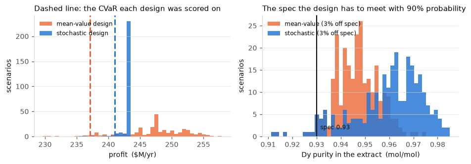
The mean-value study signs off a small section: 2.53 stages and 5.41 mol/s of organic. At the tabulated coefficients, with pH at its own optimum of 0.515, that section makes a Dy purity of 0.92999 against a 0.93 specification. It is not clear of the spec at all; it is sitting exactly on it, which is what optimizing against a single parameter vector always produces.

Now build it and run 256 campaigns. Two numbers, and the gap between them is the whole of section 7:

pH frozen where the nominal study left it — 48.8% of scenarios off spec. A coin-flip chance that the section a deterministic study called optimal cannot make the contract at all.
pH re-set per scenario — 2.7%. Comfortably inside the 10% the chance constraint allows.

Two things worth reading off that before going any further:

A design that meets its specification at the nominal parameters is not a design that meets it. Nothing about 0.92999-against-0.93 tells you what the tenth percentile does, and the tenth percentile is what the spec is written about.
What rescues this one is the operating loop, not the design. The plant is not robust; it is operated out of trouble, campaign by campaign, by a lever the deterministic study never priced. Section 7 takes the lever away and prices it.

On profit, the number to read is the one the solve was asked for: a worst decile ($\mathrm{CVaR}_{0.9}$) of $237.1M. The summary also prints a mean, an sd and a p95, but a CVaR recourse does not pin those down. Only the pH in the tail scenarios carries weight in the objective; the rest stops wherever the optimizer leaves it, so those three drift from run to run. The mean here has come out $247.7M on one execution and $247.2M on another, with the CVaR identical to six figures. Treat them as indicative, not as properties of the design.

5. The stochastic design#

t0 = time.time()
stochastic = st.solve_saa(problem, scenarios, options=options)
print(f"solved in {time.time() - t0:.1f}s\n")
print(stochastic.summary())

solved in 1.0s

SAA solution (maximize CVaR_0.9[objective] on 'profit')
  scenarios      256 (normal, seed 0)
  risk value          241.009
  mean                242.697
  sd                 0.816027
  p05 / p95           241.636 / 242.889
  first stage (one value, every scenario):
    n_stages                 3.36845
    solvent                  6.21302
  recourse (per scenario):
    variable                    mean         min         max   at bound
    pH                       0.39844     0.22101     0.57813      0.0%
  constraints (scored from the model):
    constraint                                      residual  violated
   *P(purity >= 0.93) >= 0.9 [CVaR surrogate]       6.38e-06     2.7%
  feasible: False
  note: purity fails the CVaR surrogate but meets its probability empirically. The surrogate is conservative by construction, so this design may well be acceptable -- the decision is yours, not the solver's.
  value_at_risk           -242.824
  tail_scenarios              25.6

The stochastic design is a different plant, but not in the direction section 4 was short in: 3.37 stages and 6.21 mol/s — a third more stages, 15% more solvent. Both levers go up. With the pH loop already absorbing the level, what is left to buy is margin against the ratio, and margin costs equipment.

What it buys is not a lower violation rate — that is 2.7% either way, and both designs clear the chance constraint — but the tail. The worst decile improves from $237.1M to $241.0M, which is exactly what the solve was asked to do. The two designs’ means and spreads are not compared here, for the reason given under section 4: a CVaR recourse leaves them undetermined. If the tail is not what you care about, the thing to change is the risk measure, not the solver.

Note the feasible: False and the line under it. The chance constraint is enforced through a CVaR surrogate, which is conservative by construction: this design misses the surrogate by 6e-6 while meeting the underlying probability empirically, 2.7% violated against 10% allowed. The module reports both and declines to decide which one you meant.

fig_designs(as_built, stochastic, PURITY_SPEC);

../_images/2b71882e93f8e88a93686820d83d1b4ba59d8849e91175ea3f95ffcec6beb8e1.png

fig_recourse(stochastic, scenarios, PURITY_SPEC);

../_images/3054c2a51cf8d461eb7012a830344c5d9decfdac91ead9ab70345e8c786c819a.png

aN = np.asarray(scenarios.column("a_Nd"))
aD = np.asarray(scenarios.column("a_Dy"))
level, ratio = 0.5 * (aN + aD), aD - aN
pH_chosen = np.asarray(stochastic.recourse["pH"])
purity = np.asarray(stochastic.outputs["purity"])

print(f"{'':10}{'r with pH':>12}{'r with purity':>15}")
for name, v in (("level", level), ("ratio", ratio)):
    print(f"{name:10}{np.corrcoef(pH_chosen, v)[0, 1]:12.2f}"
          f"{np.corrcoef(purity, v)[0, 1]:15.2f}")

X = np.column_stack([np.ones_like(aN), aN, aD])
resid = pH_chosen - X @ np.linalg.lstsq(X, pH_chosen, rcond=None)[0]
print(f"\npH explained by a linear fit in (a_Nd, a_Dy):"
      f"  R^2 = {1.0 - resid.var() / pH_chosen.var():.2f}")

near = ((purity >= PURITY_SPEC) & (purity < PURITY_SPEC + 0.025)).mean()
print(f"campaigns within 0.025 above spec: {near:.1%}")
print(f"campaigns below spec:              {(purity < PURITY_SPEC).mean():.1%}")

             r with pH  r with purity
level            -0.88          -0.25
ratio            -0.22           0.97

pH explained by a linear fit in (a_Nd, a_Dy):  R^2 = 1.00
campaigns within 0.025 above spec: 27.7%
campaigns below spec:              2.7%

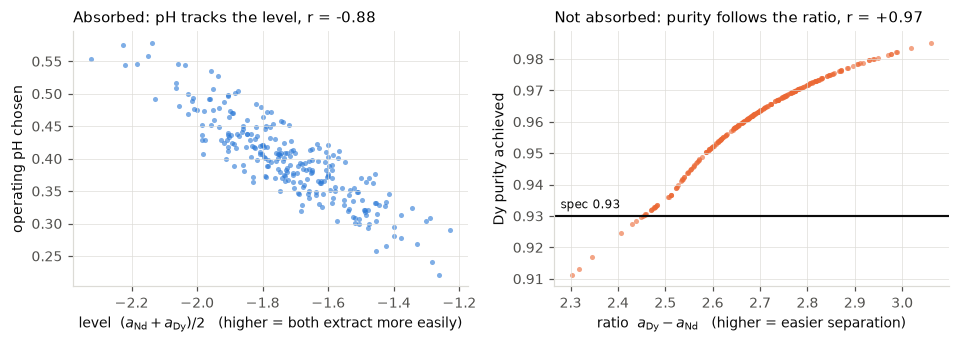
This is the most informative picture in the notebook, and it is not the one you would guess. The uncertainty has two directions and the pH loop treats them completely differently — the cell above measures it:

	absorbed by pH?	drives purity?
level, $(a_{\mathrm{Nd}} + a_{\mathrm{Dy}})/2$ — how strongly both metals extract	yes: $r(\mathrm{pH}, \text{level}) = -0.88$	barely: $r = -0.25$
ratio, $a_{\mathrm{Dy}} - a_{\mathrm{Nd}}$ — the separation factor	no: $r(\mathrm{pH}, \text{ratio}) = -0.22$	almost entirely: $r = +0.97$

The operator is running a level-compensation loop, and a very good one: when the chemistry turns out to extract more strongly than tabulated, pH comes down, and vice versa, with essentially all of the variance in the chosen pH explained by a linear fit in the two coefficients ($R^2 = 1.00$). That is why EVPI is about to come out essentially zero — the loop already does everything advance knowledge of the level would let you do, and it does it without knowing anything.

But pH cannot change the ratio. A scenario that draws a poor separation factor gets a poor purity and there is no operating move that fixes it. 28% of scenarios finish within 0.025 of the specification and 2.7% below it — that is the chance constraint doing its job, and it is the residual the loop cannot touch. It has to be carried by the design — the extra stages and the extra solvent — and carrying it is the $3.9M/yr the VSS is about to measure. The two numbers were never in tension: recourse handles one direction of the uncertainty and the design has to pay for the other.

6. Was any of this worth doing?#

Two classical numbers, and they answer different questions.

\[\mathrm{VSS} = \mathrm{EEV} - \mathrm{SP} \qquad\text{was modelling the uncertainty worth it?}\]

\[\mathrm{EVPI} = \mathrm{SP} - \mathrm{WS} \qquad\text{would measuring it be worth more?}\]

EVPI compares against the unattainable plan that knows each realization in advance, so it is an upper bound on what any measurement can possibly be worth. That makes it the number to compute before commissioning a characterization campaign.

t0 = time.time()
report = st.bounds(problem, scenarios, result=stochastic, options=options)
print(f"({time.time() - t0:.1f}s)\n")
print(report.summary())

(1.9s)

Stochastic-programming bounds
  wait and see  (WS)                       241.223
  stochastic    (SP)                       241.009
  mean-value design (EEV)                  237.135
  value of the stochastic solution           3.874
  expected value of perfect info          0.214293
  design                    mean-value    stochastic
  n_stages                     2.53483       3.36845
  solvent                      5.41499       6.21302

VSS is $3.9M/yr — 1.6% of the worst-decile profit. That is what running the stochastic program bought over the mean-value design, and on a section of this size it is worth the study, but it is not a dramatic number. It is small because the pH loop is doing so much: with an operator free to re-optimize every campaign, the mean-value design is already inside its chance constraint, and all the stochastic design can add is tail.

EVPI is $0.21M/yr — essentially zero. Perfect advance knowledge of $a_{\mathrm{Nd}}$ and $a_{\mathrm{Dy}}$ is worth almost nothing. If a lab had offered to nail those coefficients down for $1M, the answer from this run is don’t buy it — and no amount of intuition about how uncertain the chemistry is would have told you that.

The reason is again the pH loop. It absorbs the coefficient uncertainty as fast as the uncertainty arrives, so knowing it in advance adds nothing. Which raises the obvious question: what is the loop itself worth?

How much of that rests on `RHO`#

Everything above used the assumed correlation RHO = 0.75. PC88A’s refit estimates each element’s intercept separately, so the fit itself implies a correlation near zero. The diagonal sample built for the figure in section 2 (independent: same SIGMA, same seed, RHO = 0) is exactly that case. Rerun the bounds on it.

def yn(flag):
    return "yes" if flag else "no"


t0 = time.time()
report_rho0 = st.bounds(problem, independent, options=options)
eev_rho0 = st.solve_recourse(problem, independent, report_rho0.ev_first_stage,
                             options=options)
print(f"({time.time() - t0:.1f}s)\n")
W = 14
print(f"{'':30s}{'RHO = 0.75':>{W}s}{'RHO = 0':>{W}s}")
print(f"{'CVaR_0.9 of profit (SP)':30s}{report.stochastic:{W}.1f}"
      f"{report_rho0.stochastic:{W}.1f}")
print(f"{'EVPI  ($M/yr)':30s}{report.evpi:{W}.3f}{report_rho0.evpi:{W}.3f}")
print(f"{'mean-value design usable?':30s}{yn(report.ev_feasible):>{W}s}"
      f"{yn(report_rho0.ev_feasible):>{W}s}")
print(f"{'  its off-spec probability':30s}"
      f"{as_built.violation_rates[0]:{W}.1%}{eev_rho0.violation_rates[0]:{W}.1%}")
print(f"{'  its CVaR-surrogate residual':30s}"
      f"{as_built.constraint_residuals[0]:{W}.2g}"
      f"{eev_rho0.constraint_residuals[0]:{W}.2g}")
print(f"{'VSS   ($M/yr)':30s}{report.vss:{W}.1f}"
      f"{(f'{report_rho0.vss:.1f}' if report_rho0.ev_feasible else 'not a value'):>{W}s}"
      f"   (EEV - SP = {report_rho0.vss:.1f})")

(3.1s)

                                  RHO = 0.75       RHO = 0
CVaR_0.9 of profit (SP)                241.0         210.1
EVPI  ($M/yr)                          0.214         0.960
mean-value design usable?                yes            no
  its off-spec probability              2.7%          3.9%
  its CVaR-surrogate residual        5.5e-08       2.8e-06
VSS   ($M/yr)                            3.9   not a value   (EEV - SP = 37.9)

With the correlation set to what the fit implies, the part of the section 6 story that concerns the design changes. The part that concerns information holds:

The design side moves by an order of magnitude. SP falls from $241.0M to $210.1M, and EEV − SP grows from $3.9M to $37.9M/yr. The report prints not a value because the mean-value design misses the CVaR surrogate, but only by a hair: its residual of 2.8e-06 is past the 1.9e-06 tolerance and below the 6.4e-06 of the stochastic design in section 4, which was accepted. Empirically it is 3.9% off spec against 10% allowed. Read the VSS as about $38M/yr, not $3.9M.
EVPI stays small: $0.96M/yr against $0.21M. The pH loop still absorbs the level, so a lab campaign is still not worth buying.

The headline VSS is a property of the assumed RHO, not of the chemistry. Before quoting it, estimate the correlation: difflow.estimation.predicted_covariance returns it from the fit.

7. Recourse and information are substitutes#

The same problem with pH moved from recourse into first_stage: a section run at one fixed operating point, campaign after campaign, whatever the assay says. The model does not change — only which dict pH is read from.

It does get harder, and not because it has one more first-stage variable. With the loop gone, the chance constraint has to be met by the geometry alone, so the feasible region is a thin shell in (n_stages, solvent, pH) and the objective climbs steeply toward its edge. With the section 4 settings (two starts, 300 steps) the solve stops about $2.5M/yr of CVaR short of the answer below, at a point that fails the surrogate. The settings below give it eight starts and twice the steps.

rigid_options = st.SAAOptions(steps=600, rounds=8, n_starts=8)

no_recourse = st.TwoStageProblem(
    model=circuit,
    first_stage={"n_stages": (2.0, 16.0), "solvent": (3.0, 45.0),
                 "pH": (0.1, 1.2)},                    # pH is now here-and-now
    objective="profit", maximize=True, risk=("cvar", 0.9),
    constraints=[("purity", ">=", PURITY_SPEC, CONFIDENCE)],
)
t0 = time.time()
rigid = st.bounds(no_recourse, scenarios, options=rigid_options)
print(f"({time.time() - t0:.1f}s)\n")
print(rigid.summary())

(10.8s)

Stochastic-programming bounds
  wait and see  (WS)                       241.229
  stochastic    (SP)                       167.193
  mean-value design (EEV)                  228.178
  value of the stochastic solution        -60.9852
  expected value of perfect info           74.0363
  ! the mean-value design does NOT meet the constraints under the distribution, so EEV is the objective of an inadmissible design and VSS above is not a value. Read it as: ignoring the uncertainty does not produce a usable design here.
  design                    mean-value    stochastic
  n_stages                     2.53471       4.58537
  solvent                      5.40946        5.8626
  pH                          0.515274      0.375135

print(f"{'':26s}{'with a pH loop':>16s}{'without one':>16s}")
print(f"{'CVaR_0.9 of profit':26s}{report.stochastic:16.1f}"
      f"{rigid.stochastic:16.1f}")
print(f"{'EVPI  ($M/yr)':26s}{report.evpi:16.3f}{rigid.evpi:16.1f}")
print(f"{'mean-value design usable?':26s}{yn(report.ev_feasible):>16s}"
      f"{yn(rigid.ev_feasible):>16s}")
# VSS compares against the mean-value design, so it is a value only when that
# design is one you could actually build.
print(f"{'VSS   ($M/yr)':26s}{report.vss:16.1f}"
      f"{(f'{rigid.vss:.1f}' if rigid.ev_feasible else 'not a value'):>16s}")
print()
print(f"The pH loop is worth {report.stochastic - rigid.stochastic:,.1f} $M/yr "
      f"of CVaR; EVPI without it is {rigid.evpi:,.1f}.")

                            with a pH loop     without one
CVaR_0.9 of profit                   241.0           167.2
EVPI  ($M/yr)                        0.214            74.0
mean-value design usable?              yes              no
VSS   ($M/yr)                          3.9     not a value

The pH loop is worth 73.8 $M/yr of CVaR; EVPI without it is 74.0.

fig_bounds(report, rigid);

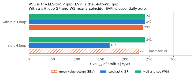
../_images/894808458d7fe20050e4ee5f2f44158cecbb38b37d3aead7f21db28268fef6b1.png

Taking the loop away costs $73.8M/yr of CVaR — 241.0 with it, 167.2 without — and that is the optimistic reading, because it compares two designs that both clear the chance constraint. The mean-value design does not: at the rigid problem’s mean-value point the section scores 228.2, better than either, by being off spec in 49% of scenarios. bounds says so rather than reporting the difference as a negative VSS, which is why the table above prints not a value in that column instead of $-61M.

That is the whole lesson of the two numbers, quantified:

With a working pH loop, information about $D$ is worth $0.21M/yr — the loop already handles it. Do not fund the characterization campaign.
Without one, information is worth $74M/yr — but so is the loop, which is the same $74M and is almost certainly cheaper than resolving the chemistry.

Recourse and information are substitutes, and the cheap one usually wins. Neither number is available from a deterministic study, or from propagating uncertainty through a fixed design; they exist only once the design itself is optimized against the distribution.

8. Do not trust it until it has been checked#

A stochastic program will return a confident answer to a badly posed question. check_scenario_health is the counterpart of check_delta_health in difflow.planning: the things that go quietly wrong, each with a number.

health = st.check_scenario_health(problem, scenarios, stochastic)
print(health.summary())

Scenario health: 256 scenarios
  risk value               241.009  +/- 0.479 (sampling)
  half-sample risk         240.266
  CVaR tail                   25.6  scenarios
  first-stage lever             dRisk/dx
  n_stages                     -0.390754
  solvent                         1.5775
  findings: none

Both levers have live gradients — no clip or where has flattened one into a dead column — the CVaR tail holds 26 scenarios rather than two, the recourse is not pinned at a bound, and the half-sample risk is within two bootstrap standard errors of the full sample (1.5 se here), the threshold at which check_scenario_health warns.

The formal version is the Mak–Morton–Wood replication bound: solve on several independent samples for a bound from the optimistic side, evaluate the candidate on one large independent sample for a bound from the achievable side, and report the gap with a confidence limit. It is the only place in the module that deliberately redraws the sample.

t0 = time.time()
gap = st.optimality_gap(problem, scenarios, stochastic, n_replications=4,
                        n_evaluation=1024, options=options)
print(f"({time.time() - t0:.1f}s)\n")
print(gap.summary())

(6.5s)

SAA optimality gap (4 replications, 1024-scenario evaluation)
  candidate value               240.536
  replication bound             240.974
  gap                          0.438305  +/- 0.621
  95% one-sided limit           1.90005
  i.e. the design is within 1.90005 of the true optimum with 95% confidence.

The bound is loose, and honestly so: with four replications the standard error is larger than the gap itself. That is a statement about the sample size, not about the design — and it is exactly the kind of thing that a single confident number would have hidden. Raise n_replications, and the scenario count n in from_covariance, to tighten it, at linear cost; n_evaluation sets the size of the candidate’s evaluation sample.

What to take away#

Correlation between fitted coefficients is not a detail. Treating $a_{\mathrm{Nd}}$ and $a_{\mathrm{Dy}}$ as independent doubled the apparent uncertainty in the separation factor, and assuming a correlation your fit did not produce does the reverse. Here, replacing the assumed 0.75 with the 0 that PC88A’s per-element fit implies takes the VSS from $3.9M to about $38M/yr. Use ScenarioSet.from_covariance with the covariance your fit actually produced.
Clearing a specification at the nominal parameters says nothing about the tail. The mean-value design met the 0.93 spec to four figures (0.92999) at the nominal coefficients and, held at that pH, missed the spec in 49% of scenarios. Letting the operator re-optimize pH each campaign took the same geometry to 2.7%, because pH moves the level and purity follows the ratio.
VSS says whether to keep doing this. Here it is $3.9M/yr, small precisely because the pH loop absorbs most of what the stochastic design would otherwise have to buy with steel. A small VSS is a perfectly good answer, and finding it early saves the study — as is no VSS, which is what comes back when the mean-value design cannot meet the constraints at all.
EVPI is the ceiling on what a measurement can be worth, and it collapses when recourse can already absorb the uncertainty. Compute it before commissioning the campaign.
Check the sample before believing the answer. Dead levers, an empty CVaR tail and saturated recourse all produce confident nonsense.

Where to go next#

docs/stochastic.md — the module, its three implementation choices, and what is deliberately out of scope.
difflow.flexibility — when you want a guarantee over an envelope rather than a probability over a sample. Its expected_feasibility is the cheap first look at a design you already have.
difflow.planning.backoff — the linear-model answer: propagate the covariance onto the constraint and buy kappa * sigma of margin. Orders of magnitude cheaper, and right whenever the constraint is nearly linear over the spread.
difflow.estimation — where the covariance used here should come from.

	absorbed by pH?	drives purity?
level, \((a_{\mathrm{Nd}} + a_{\mathrm{Dy}})/2\) — how strongly both metals extract	yes: \(r(\mathrm{pH}, \text{level}) = -0.88\)	barely: \(r = -0.25\)
ratio, \(a_{\mathrm{Dy}} - a_{\mathrm{Nd}}\) — the separation factor	no: \(r(\mathrm{pH}, \text{ratio}) = -0.22\)	almost entirely: \(r = +0.97\)

Stochastic Programming: Nd/Dy Separation with Uncertain Distribution Coefficients

Contents

Stochastic Programming: Nd/Dy Separation with Uncertain Distribution Coefficients#

Before any number in here is copied#

1. Setup#

Figures#

2. Putting a distribution on \(D\)#

3. The model#

The split that is the whole model#

4. The problem, and the design you get by ignoring the uncertainty#

5. The stochastic design#

6. Was any of this worth doing?#

How much of that rests on `RHO`#

7. Recourse and information are substitutes#

8. Do not trust it until it has been checked#

What to take away#

Where to go next#

Stochastic Programming: Nd/Dy Separation with Uncertain Distribution Coefficients

Contents

Stochastic Programming: Nd/Dy Separation with Uncertain Distribution Coefficients#

Before any number in here is copied#

1. Setup#

Figures#

2. Putting a distribution on \(D\)#

3. The model#

The split that is the whole model#

4. The problem, and the design you get by ignoring the uncertainty#

5. The stochastic design#

6. Was any of this worth doing?#

How much of that rests on RHO#

7. Recourse and information are substitutes#

8. Do not trust it until it has been checked#

What to take away#

Where to go next#

How much of that rests on `RHO`#