Dynamic Modeling with difflow

This notebook demonstrates the dynamic (transient) simulation capabilities of difflow.

Topics covered:

1. Basic ODE integration

2. Dynamic CSTR simulation (startup)

3. Dynamic flowsheets (multi-unit)

4. DAE systems (flash drum with VLE)

5. Diffrax backend for stiff systems

6. Gradient-based optimization of dynamic systems

import jax
import jax.numpy as jnp
import matplotlib.pyplot as plt

# Configure JAX
jax.config.update("jax_enable_x64", True)

# Import difflow dynamic module
from difflow.dynamic import (
    integrate,
    integrate_unit,
    DynamicCSTR,
    DynamicTank,
    DynamicFlowsheet,
    integrate_dae,
    DynamicFlashDrum,
)
from difflow.streams import make_stream

WARNING:2026-03-01 07:51:08,778:jax._src.xla_bridge:905: Platform 'mps' is experimental and not all JAX functionality may be correctly supported!

WARNING:2026-03-01 07:51:08,810:jax._src.xla_bridge:905: Platform 'METAL' is experimental and not all JAX functionality may be correctly supported!

WARNING: All log messages before absl::InitializeLog() is called are written to STDERR
W0000 00:00:1772369468.810913 12639203 mps_client.cc:510] WARNING: JAX Apple GPU support is experimental and not all JAX functionality is correctly supported!
I0000 00:00:1772369468.811151 12639203 service.cc:145] XLA service 0xa57af8300 initialized for platform METAL (this does not guarantee that XLA will be used). Devices:
I0000 00:00:1772369468.811157 12639203 service.cc:153]   StreamExecutor device (0): Metal, <undefined>
I0000 00:00:1772369468.811954 12639203 mps_client.cc:406] Using Simple allocator.
I0000 00:00:1772369468.811964 12639203 mps_client.cc:384] XLA backend will use up to 55662313472 bytes on device 0 for SimpleAllocator.

Metal device set to: Apple M4 Pro

1. Basic ODE Integration

The integrate() function provides a unified interface for solving ODEs.

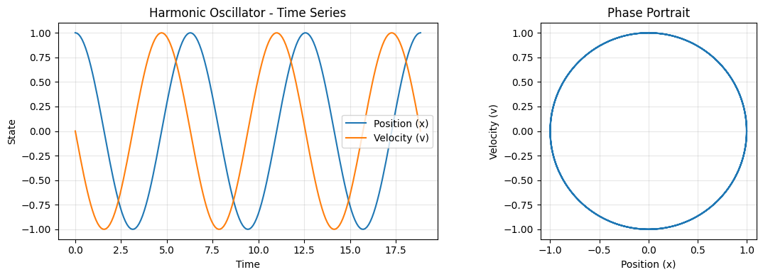
Example: Harmonic Oscillator

The harmonic oscillator is described by: $\(\frac{d^2x}{dt^2} = -x\)$

As a first-order system: $\(\frac{dx}{dt} = v, \quad \frac{dv}{dt} = -x\)$

def harmonic_oscillator(t, y):
    """Harmonic oscillator: d²x/dt² = -x"""
    x, v = y[0], y[1]
    return jnp.array([v, -x])

# Initial conditions: x=1, v=0
y0 = jnp.array([1.0, 0.0])

# Integrate for 3 periods
result = integrate(
    harmonic_oscillator,
    y0,
    t_span=(0.0, 6 * jnp.pi),
    method="RK4",
    n_steps=200,
)

print(f"Final state: x={result.y_final[0]:.4f}, v={result.y_final[1]:.4f}")
print(f"Steps taken: {result.info.n_steps}")

Final state: x=1.0000, v=0.0000
Steps taken: 200

# Plot the trajectory
fig, (ax1, ax2) = plt.subplots(1, 2, figsize=(12, 4))

# Time series
ax1.plot(result.trajectory.t, result.trajectory.y[:, 0], label='Position (x)')
ax1.plot(result.trajectory.t, result.trajectory.y[:, 1], label='Velocity (v)')
ax1.set_xlabel('Time')
ax1.set_ylabel('State')
ax1.set_title('Harmonic Oscillator - Time Series')
ax1.legend()
ax1.grid(True, alpha=0.3)

# Phase portrait
ax2.plot(result.trajectory.y[:, 0], result.trajectory.y[:, 1])
ax2.set_xlabel('Position (x)')
ax2.set_ylabel('Velocity (v)')
ax2.set_title('Phase Portrait')
ax2.set_aspect('equal')
ax2.grid(True, alpha=0.3)

plt.tight_layout()
plt.show()

Example: Exponential Decay

\[\frac{dy}{dt} = -ky\]

Exact solution: \(y(t) = y_0 e^{-kt}\)

k = 0.5  # Decay rate

def exponential_decay(t, y):
    return -k * y

y0 = jnp.array([1.0])
t_span = (0.0, 5.0)

# Compare methods
methods = ["Euler", "RK4", "RK45"]
results = {}

for method in methods:
    if method == "RK45":
        results[method] = integrate(exponential_decay, y0, t_span, method=method, rtol=1e-6)
    else:
        results[method] = integrate(exponential_decay, y0, t_span, method=method, n_steps=50)

# Exact solution
t_exact = jnp.linspace(0, 5, 100)
y_exact = jnp.exp(-k * t_exact)

# Plot
plt.figure(figsize=(10, 5))
plt.plot(t_exact, y_exact, 'k-', linewidth=2, label='Exact')

for method, result in results.items():
    plt.plot(result.trajectory.t, result.trajectory.y[:, 0], 'o-', 
             markersize=4, alpha=0.7, label=f'{method}')

plt.xlabel('Time')
plt.ylabel('y')
plt.title('Exponential Decay - Method Comparison')
plt.legend()
plt.grid(True, alpha=0.3)
plt.show()

# Print final errors
y_exact_final = float(jnp.exp(-k * t_span[1]))
print("Final value errors:")
for method, result in results.items():
    error = abs(float(result.y_final[0]) - y_exact_final)
    print(f"  {method}: {error:.2e}")

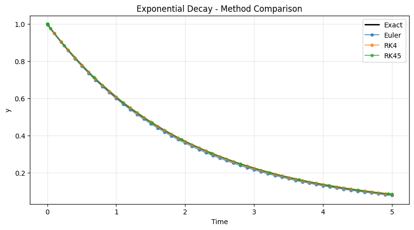
Final value errors:
  Euler: 5.14e-03
  RK4: 1.11e-08
  RK45: 9.15e-08

2. Dynamic CSTR Simulation

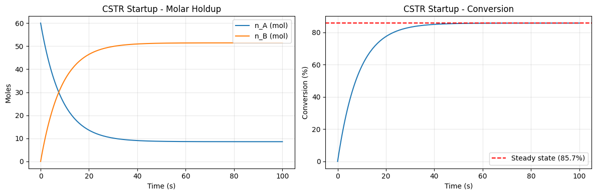
Simulate the startup of a CSTR with reaction A → B.

# Define reaction kinetics: r = k * C_A
def rate_fn(C, T, params):
    k = params["k"]
    return jnp.array([k * C["A"]])

# Stoichiometry: A → B
stoich = jnp.array([
    [-1.0],  # A consumed
    [+1.0],  # B produced
])

# Create dynamic CSTR
cstr = DynamicCSTR(
    volume=1.0,  # m³
    rate_fn=rate_fn,
    stoich=stoich,
    species_order=["A", "B"],
    rate_params={"k": 0.1},  # rate constant (1/s)
    name="reactor",
)

print(f"CSTR state variables: {cstr.state_spec().names}")
print(f"Number of states: {cstr.state_spec().n_states}")

CSTR state variables: ['n_A', 'n_B']
Number of states: 2

# Create inlet stream
inlet = make_stream({"A": 1.0, "B": 0.0}, T=350.0, P=101325.0)
print(f"Inlet: F_A={inlet['F_A']:.2f} mol/s, F_B={inlet['F_B']:.2f} mol/s")

# Simulate startup (from initial state based on inlet)
result = integrate_unit(
    cstr,
    inputs={"inlet": inlet},
    t_span=(0.0, 100.0),  # 100 seconds
    method="RK4",
    n_steps=200,
)

print(f"\nFinal state:")
print(f"  n_A = {result.y_final[0]:.4f} mol")
print(f"  n_B = {result.y_final[1]:.4f} mol")
print(f"  Total moles = {result.y_final[0] + result.y_final[1]:.4f} mol")

Inlet: F_A=1.00 mol/s, F_B=0.00 mol/s

Final state:
  n_A = 8.5719 mol
  n_B = 51.4281 mol
  Total moles = 60.0000 mol

# Plot CSTR dynamics
fig, (ax1, ax2) = plt.subplots(1, 2, figsize=(12, 4))

# Molar holdup
ax1.plot(result.trajectory.t, result.trajectory.y[:, 0], label='n_A (mol)')
ax1.plot(result.trajectory.t, result.trajectory.y[:, 1], label='n_B (mol)')
ax1.set_xlabel('Time (s)')
ax1.set_ylabel('Moles')
ax1.set_title('CSTR Startup - Molar Holdup')
ax1.legend()
ax1.grid(True, alpha=0.3)

# Conversion
n_A = result.trajectory.y[:, 0]
n_B = result.trajectory.y[:, 1]
conversion = n_B / (n_A + n_B + 1e-10)  # Mole fraction of B = conversion

ax2.plot(result.trajectory.t, conversion * 100)
ax2.set_xlabel('Time (s)')
ax2.set_ylabel('Conversion (%)')
ax2.set_title('CSTR Startup - Conversion')
ax2.grid(True, alpha=0.3)

# Steady-state conversion (analytical)
# For CSTR: X = k*tau / (1 + k*tau) where tau = n_total / F_total
# At steady state, n_total ≈ 60 mol (from initial_state: tau=60s * F=1 mol/s)
# F_total = 1.0 mol/s
k = 0.1
tau = 60.0  # residence time = holdup / flow rate
X_ss = k * tau / (1 + k * tau)
ax2.axhline(X_ss * 100, color='r', linestyle='--', label=f'Steady state ({X_ss*100:.1f}%)')
ax2.legend()

plt.tight_layout()
plt.show()

3. Dynamic Flowsheet

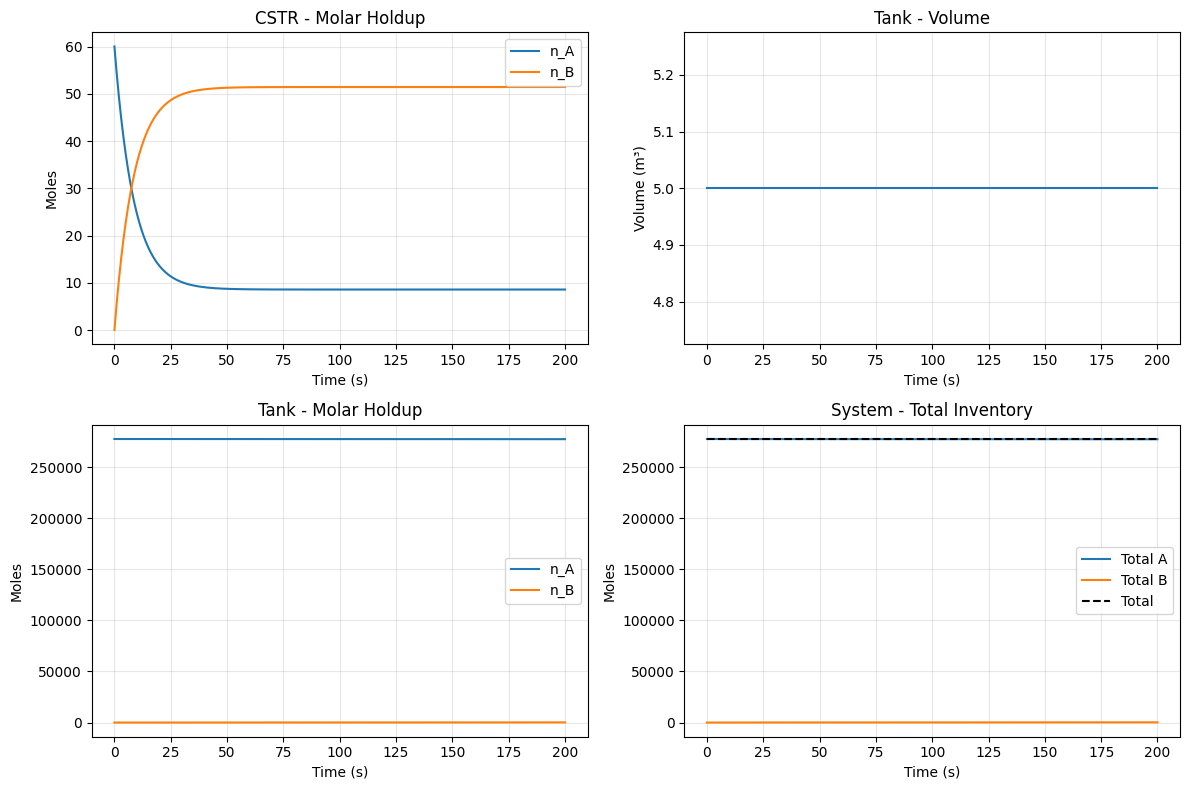
Connect multiple units: CSTR → Storage Tank

# Create a storage tank
tank = DynamicTank(
    max_volume=10.0,  # m³
    species_order=["A", "B"],
    name="storage",
)

# Build flowsheet
fs = DynamicFlowsheet(species_order=["A", "B"])

# Add feed
feed = make_stream({"A": 1.0, "B": 0.0}, T=350.0, P=101325.0)
fs.add_feed("feed", feed)

# Add units
fs.add_unit(cstr, inlet_names=["feed"], outlet_names=["reactor_out"])
fs.add_unit(tank, inlet_names=["reactor_out"], outlet_names=["product"])

print(f"Flowsheet units: {[u.name for u in fs._units]}")
print(f"Total states: {sum(u.unit.state_spec().n_states for u in fs._units)}")

Flowsheet units: ['reactor', 'storage']
Total states: 5

# Simulate flowsheet
result = fs.simulate(
    t_span=(0.0, 200.0),
    method="RK4",
    n_steps=400,
)

print(f"Final combined state: {result.y_final}")
print(f"Success: {result.info.success}")

Final combined state: [8.57142858e+00 5.14285714e+01 5.00000000e+00 2.77335975e+05
 1.64024938e+02]
Success: True

# Extract per-unit states
# CSTR: states 0-1 (n_A, n_B)
# Tank: states 2-4 (V, n_A, n_B)
cstr_states = result.trajectory.y[:, :2]
tank_states = result.trajectory.y[:, 2:]

fig, axes = plt.subplots(2, 2, figsize=(12, 8))

# CSTR moles
axes[0, 0].plot(result.trajectory.t, cstr_states[:, 0], label='n_A')
axes[0, 0].plot(result.trajectory.t, cstr_states[:, 1], label='n_B')
axes[0, 0].set_xlabel('Time (s)')
axes[0, 0].set_ylabel('Moles')
axes[0, 0].set_title('CSTR - Molar Holdup')
axes[0, 0].legend()
axes[0, 0].grid(True, alpha=0.3)

# Tank volume
axes[0, 1].plot(result.trajectory.t, tank_states[:, 0])
axes[0, 1].set_xlabel('Time (s)')
axes[0, 1].set_ylabel('Volume (m³)')
axes[0, 1].set_title('Tank - Volume')
axes[0, 1].grid(True, alpha=0.3)

# Tank moles
axes[1, 0].plot(result.trajectory.t, tank_states[:, 1], label='n_A')
axes[1, 0].plot(result.trajectory.t, tank_states[:, 2], label='n_B')
axes[1, 0].set_xlabel('Time (s)')
axes[1, 0].set_ylabel('Moles')
axes[1, 0].set_title('Tank - Molar Holdup')
axes[1, 0].legend()
axes[1, 0].grid(True, alpha=0.3)

# Total system inventory
total_A = cstr_states[:, 0] + tank_states[:, 1]
total_B = cstr_states[:, 1] + tank_states[:, 2]
axes[1, 1].plot(result.trajectory.t, total_A, label='Total A')
axes[1, 1].plot(result.trajectory.t, total_B, label='Total B')
axes[1, 1].plot(result.trajectory.t, total_A + total_B, 'k--', label='Total')
axes[1, 1].set_xlabel('Time (s)')
axes[1, 1].set_ylabel('Moles')
axes[1, 1].set_title('System - Total Inventory')
axes[1, 1].legend()
axes[1, 1].grid(True, alpha=0.3)

plt.tight_layout()
plt.show()

4. DAE Systems

Differential-Algebraic Equations combine ODEs with algebraic constraints.

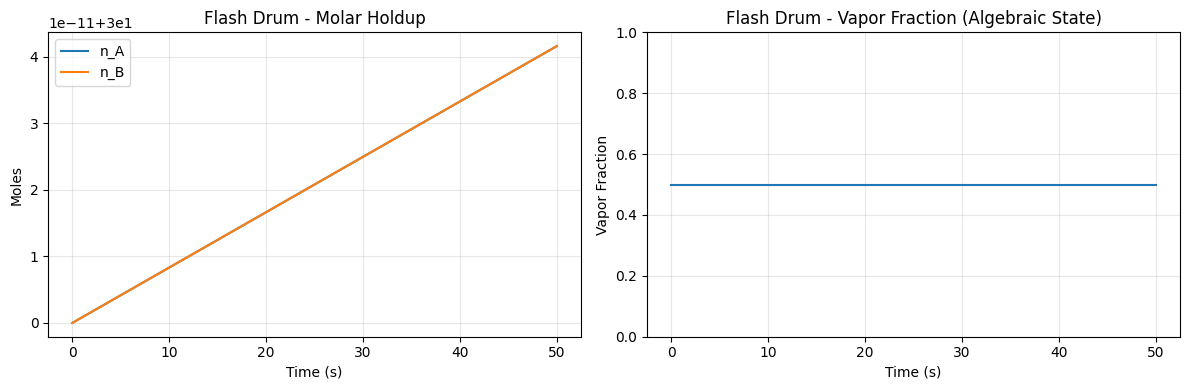
Example: Flash drum where vapor-liquid equilibrium must be satisfied at each time step.

# Create flash drum with VLE equilibrium
# K_func returns K-values for each species given temperature
def K_func(T):
    # Simple constant K-values: A is more volatile (K=2), B less (K=0.5)
    return jnp.array([2.0, 0.5])

flash = DynamicFlashDrum(
    volume=1.0,
    species_order=["A", "B"],
    K_func=K_func,
    name="flash",
)

print(f"Differential states: {flash.state_spec().names}")
print(f"Algebraic states: {flash.algebraic_spec().names}")

Differential states: ['n_A', 'n_B', 'H']
Algebraic states: ['beta']

# Feed with 50/50 mixture
flash_feed = make_stream({"A": 0.5, "B": 0.5}, T=350.0, P=101325.0)

# Integrate DAE
dae_result = integrate_dae(
    flash,
    inputs={"inlet": flash_feed},
    t_span=(0.0, 50.0),
    method="RK4",
    n_steps=100,
)

print(f"Final differential states (moles): {dae_result.x_final}")
print(f"Final algebraic states (V_frac): {dae_result.z_final}")

Final differential states (moles): [30. 30.  0.]
Final algebraic states (V_frac): [0.5]

# Plot DAE results
fig, (ax1, ax2) = plt.subplots(1, 2, figsize=(12, 4))

# Molar holdup
ax1.plot(dae_result.t_history, dae_result.x_history[:, 0], label='n_A')
ax1.plot(dae_result.t_history, dae_result.x_history[:, 1], label='n_B')
ax1.set_xlabel('Time (s)')
ax1.set_ylabel('Moles')
ax1.set_title('Flash Drum - Molar Holdup')
ax1.legend()
ax1.grid(True, alpha=0.3)

# Vapor fraction (algebraic variable)
ax2.plot(dae_result.t_history, dae_result.z_history[:, 0])
ax2.set_xlabel('Time (s)')
ax2.set_ylabel('Vapor Fraction')
ax2.set_title('Flash Drum - Vapor Fraction (Algebraic State)')
ax2.set_ylim([0, 1])
ax2.grid(True, alpha=0.3)

plt.tight_layout()
plt.show()

5. Diffrax Backend

For advanced solvers (adaptive step, stiff systems), use the diffrax backend.

# Check if diffrax is available
from difflow.dynamic import check_diffrax_available, list_diffrax_solvers

if check_diffrax_available():
    print("Diffrax is available!")
    print(f"Available solvers: {list_diffrax_solvers()}")
else:
    print("Diffrax not installed. Install with: pip install diffrax")

Diffrax is available!
Available solvers: ['bosh3', 'dopri5', 'dopri8', 'euler', 'heun', 'implicit_euler', 'kvaerno3', 'kvaerno4', 'kvaerno5', 'leapfrog_midpoint', 'midpoint', 'ralston', 'semi_implicit_euler', 'tsit5']

# Example: Using adaptive solvers for better accuracy
if check_diffrax_available():
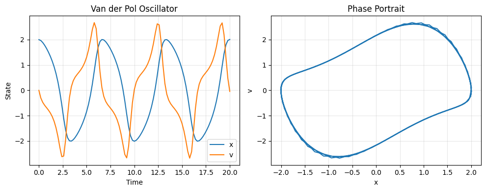
    # Van der Pol oscillator - a moderately stiff oscillator
    # mu controls stiffness - higher values make it stiffer
    mu = 1.0  # Moderate stiffness
    
    def vanderpol(t, y):
        x, v = y[0], y[1]
        dx = v
        dv = mu * (1 - x**2) * v - x
        return jnp.array([dx, dv])

    y0 = jnp.array([2.0, 0.0])

    # Use adaptive Dopri5 solver
    result = integrate(
        vanderpol, y0,
        t_span=(0.0, 20.0),
        method="diffrax:dopri5",
        rtol=1e-6, atol=1e-8,
    )

    print(f"Final state: x={result.y_final[0]:.4f}, v={result.y_final[1]:.4f}")
    print(f"Steps taken: {result.info.n_steps}")
    
    # Plot phase portrait
    plt.figure(figsize=(10, 4))
    plt.subplot(1, 2, 1)
    plt.plot(result.trajectory.t, result.trajectory.y[:, 0], label='x')
    plt.plot(result.trajectory.t, result.trajectory.y[:, 1], label='v')
    plt.xlabel('Time')
    plt.ylabel('State')
    plt.title('Van der Pol Oscillator')
    plt.legend()
    plt.grid(True, alpha=0.3)
    
    plt.subplot(1, 2, 2)
    plt.plot(result.trajectory.y[:, 0], result.trajectory.y[:, 1])
    plt.xlabel('x')
    plt.ylabel('v')
    plt.title('Phase Portrait')
    plt.grid(True, alpha=0.3)
    plt.tight_layout()
    plt.show()
else:
    print("Skipping example (diffrax not installed)")

Final state: x=2.0081, v=-0.0425
Steps taken: 219

# Compare different explicit solvers on mildly stiff problem
if check_diffrax_available():
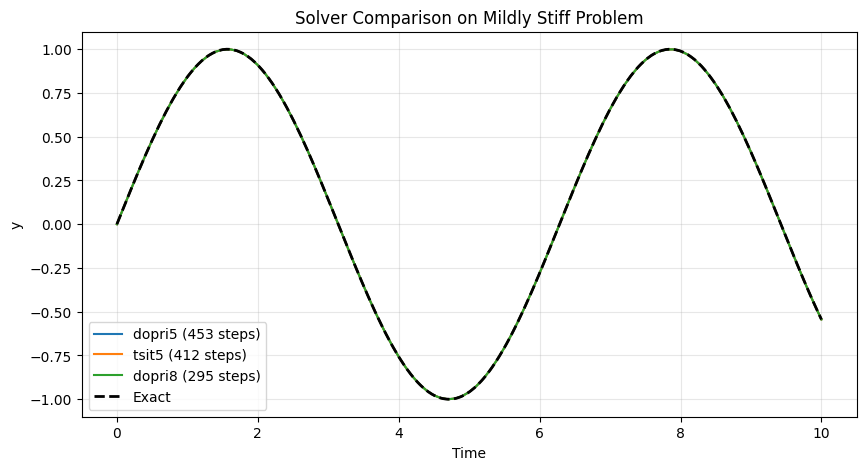
    # Mildly stiff decay: y' = -100*(y - sin(t)) + cos(t)
    # Exact solution: y = sin(t)
    def stiff_decay(t, y):
        return -100 * (y - jnp.sin(t)) + jnp.cos(t)

    y0 = jnp.array([0.0])
    t_span = (0.0, 10.0)

    # Compare explicit adaptive solvers
    solvers = ["dopri5", "tsit5", "dopri8"]
    results = {}

    for solver in solvers:
        results[solver] = integrate(
            stiff_decay, y0, t_span,
            method=f"diffrax:{solver}",
            rtol=1e-5, atol=1e-7,
        )

    # Plot
    plt.figure(figsize=(10, 5))
    for solver, result in results.items():
        plt.plot(result.trajectory.t, result.trajectory.y[:, 0], 
                 label=f'{solver} ({result.info.n_steps} steps)')

    # Exact solution: y = sin(t)
    t_exact = jnp.linspace(0, 10, 200)
    plt.plot(t_exact, jnp.sin(t_exact), 'k--', linewidth=2, label='Exact')

    plt.xlabel('Time')
    plt.ylabel('y')
    plt.title('Solver Comparison on Mildly Stiff Problem')
    plt.legend()
    plt.grid(True, alpha=0.3)
    plt.show()

6. Gradient-Based Optimization

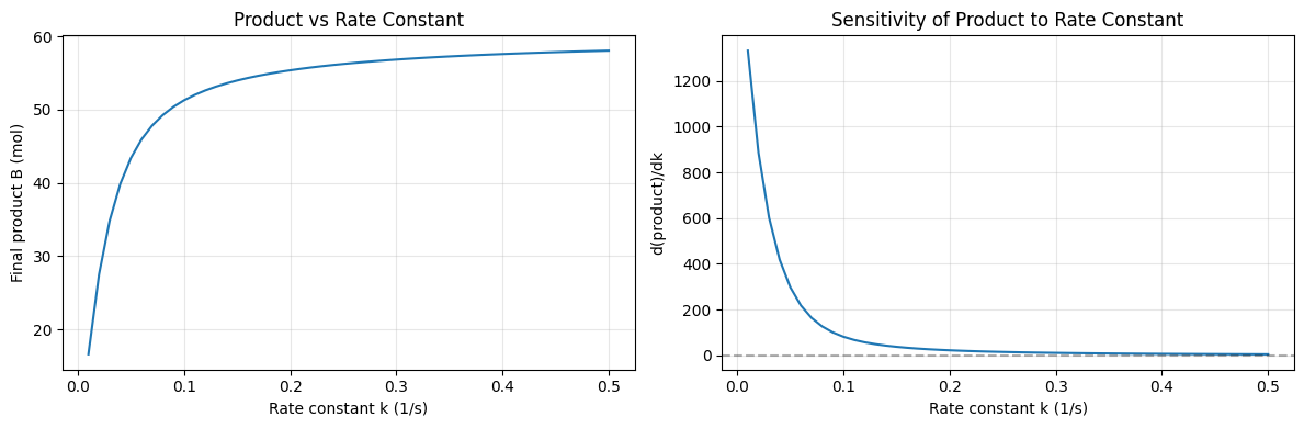
All dynamic simulations are differentiable via JAX autodiff.

# Optimize rate constant to maximize conversion
def simulate_cstr(k):
    """Simulate CSTR with rate constant k, return final product."""
    def rate_fn(C, T, params):
        return jnp.array([k * C["A"]])

    cstr = DynamicCSTR(
        volume=1.0,
        rate_fn=rate_fn,
        stoich=jnp.array([[-1.0], [1.0]]),
        species_order=["A", "B"],
        rate_params={},
    )

    inlet = make_stream({"A": 1.0, "B": 0.0}, T=350.0, P=101325.0)
    result = integrate_unit(cstr, {"inlet": inlet}, (0.0, 50.0), method="RK4", n_steps=100)
    
    # Return final B amount
    return result.y_final[1]

# Compute gradient
k_val = jnp.array(0.1)
product = simulate_cstr(k_val)
grad_k = jax.grad(simulate_cstr)(k_val)

print(f"At k = {k_val}:")
print(f"  Final product: {product:.4f} mol")
print(f"  d(product)/dk: {grad_k:.4f}")

At k = 0.1:
  Final product: 51.2780 mol
  d(product)/dk: 80.7842

# Parameter sensitivity analysis
k_values = jnp.linspace(0.01, 0.5, 50)
products = jax.vmap(simulate_cstr)(k_values)
gradients = jax.vmap(jax.grad(simulate_cstr))(k_values)

fig, (ax1, ax2) = plt.subplots(1, 2, figsize=(12, 4))

ax1.plot(k_values, products)
ax1.set_xlabel('Rate constant k (1/s)')
ax1.set_ylabel('Final product B (mol)')
ax1.set_title('Product vs Rate Constant')
ax1.grid(True, alpha=0.3)

ax2.plot(k_values, gradients)
ax2.set_xlabel('Rate constant k (1/s)')
ax2.set_ylabel('d(product)/dk')
ax2.set_title('Sensitivity of Product to Rate Constant')
ax2.axhline(0, color='k', linestyle='--', alpha=0.3)
ax2.grid(True, alpha=0.3)

plt.tight_layout()
plt.show()

# Gradient descent to find optimal k for target conversion
import optax  # Use adaptive optimizer for better convergence

def loss(k):
    """Squared error from target product amount."""
    target = 45.0  # Target 45 mol of B (achievable in range k=0.01-0.5)
    product = simulate_cstr(k)
    return (product - target)**2

# Use Adam optimizer for adaptive learning rates
optimizer = optax.adam(learning_rate=0.01)
k = jnp.array(0.3)  # Initial guess - start high to see decrease
opt_state = optimizer.init(k)
history = []

print("Gradient descent optimization of rate constant k:")
print("-" * 50)

for i in range(100):
    l = loss(k)
    g = jax.grad(loss)(k)
    updates, opt_state = optimizer.update(g, opt_state, k)
    k = optax.apply_updates(k, updates)
    k = jnp.clip(k, 0.01, 1.0)  # Keep k in valid range
    history.append((float(k), float(l)))
    
    if (i + 1) % 20 == 0:
        print(f"  Iter {i+1:3d}: k = {float(k):.4f}, loss = {float(l):.2f}")

print(f"\nOptimal k: {k:.4f}")
print(f"Final product: {simulate_cstr(k):.2f} mol (target: 45.0)")

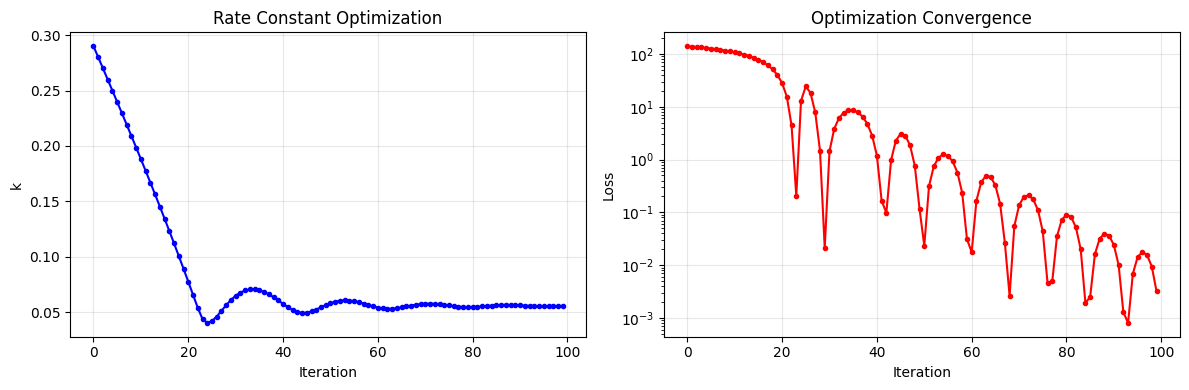
# Plot optimization
fig, (ax1, ax2) = plt.subplots(1, 2, figsize=(12, 4))

ax1.plot([h[0] for h in history], 'b-o', markersize=3)
ax1.set_xlabel('Iteration')
ax1.set_ylabel('k')
ax1.set_title('Rate Constant Optimization')
ax1.grid(True, alpha=0.3)

ax2.semilogy([h[1] for h in history], 'r-o', markersize=3)
ax2.set_xlabel('Iteration')
ax2.set_ylabel('Loss')
ax2.set_title('Optimization Convergence')
ax2.grid(True, alpha=0.3)

plt.tight_layout()
plt.show()

Gradient descent optimization of rate constant k:
--------------------------------------------------

  Iter  20: k = 0.0892, loss = 40.17

  Iter  40: k = 0.0607, loss = 2.85

  Iter  60: k = 0.0554, loss = 0.03

  Iter  80: k = 0.0547, loss = 0.07

  Iter 100: k = 0.0559, loss = 0.00

Optimal k: 0.0559
Final product: 44.99 mol (target: 45.0)

Summary

The difflow.dynamic module provides:

1. Unified ODE integration via integrate() with multiple methods (RK4, RK45, Euler, diffrax)

2. Dynamic unit operations (DynamicCSTR, DynamicTank) implementing the DynamicUnit protocol

3. Multi-unit flowsheets via DynamicFlowsheet for connected process simulation

4. DAE support for systems with algebraic constraints (VLE, etc.)

5. Advanced solvers via diffrax backend for stiff systems

6. Full differentiability enabling gradient-based optimization of dynamic systems

See docs/dynamic-modeling.md for complete API documentation.