
Optimistix: Nonlinear Solvers in JAX#
Optimistix is a JAX library for root finding, minimization, least squares, and fixed-point iteration. All solvers are:
Fully differentiable (gradients through the solve)
JIT-compilable
Compatible with vmap for batched problems
What You’ll Learn#
Root finding (solving f(x) = 0)
Fixed-point iteration (solving x = g(x))
Minimization (finding argmin f(x))
Least squares (fitting models to data)
Implicit differentiation
Chemical engineering applications
import jax
import jax.numpy as jnp
from jax import grad, jit, vmap
import optimistix as optx
import matplotlib.pyplot as plt

jax.config.update("jax_enable_x64", True)

print(f"JAX version: {jax.__version__}")
print(f"Optimistix version: {optx.__version__}")
WARNING:2026-01-10 20:28:52,018:jax._src.xla_bridge:852: An NVIDIA GPU may be present on this machine, but a CUDA-enabled jaxlib is not installed. Falling back to cpu.
JAX version: 0.8.2
Optimistix version: 0.0.11
1. Root Finding#
Find \(x\) such that \(f(x) = 0\).
Available Root Finders#
Solver |
Method |
Best For |
|---|---|---|
|
Newton-Raphson |
Smooth functions, fast convergence |
|
Chord method |
When Jacobian is expensive |
|
Bisection |
1D problems, guaranteed convergence |
|
Brent’s method |
1D problems, no derivatives needed |
# Example: Solve x³ - x - 2 = 0
def f(x, args):
    return x**3 - x - 2

# Newton's method
solver = optx.Newton(rtol=1e-8, atol=1e-8)
x0 = jnp.array(1.5)  # Initial guess

solution = optx.root_find(f, solver, x0)

print(f"Root: x = {float(solution.value):.10f}")
print(f"f(x) = {float(f(solution.value, None)):.2e}")
print(f"Converged: {solution.result == optx.RESULTS.successful}")
Root: x = 1.5213797068
f(x) = 0.00e+00
Converged: True
# Multivariate root finding
def system(xy, args):
    """System of nonlinear equations:
    x² + y² = 4
    x*y = 1
    """
    x, y = xy
    return jnp.array([
        x**2 + y**2 - 4,
        x * y - 1
    ])

solver = optx.Newton(rtol=1e-10, atol=1e-10)
x0 = jnp.array([1.5, 1.0])  # Initial guess

solution = optx.root_find(system, solver, x0)

print(f"Solution: x = {solution.value[0]:.6f}, y = {solution.value[1]:.6f}")
print(f"Residual: {jnp.linalg.norm(system(solution.value, None)):.2e}")

# Verify
x, y = solution.value
print(f"\nVerification:")
print(f"  x² + y² = {x**2 + y**2:.6f} (should be 4)")
print(f"  x * y = {x * y:.6f} (should be 1)")
Solution: x = 1.931852, y = 0.517638
Residual: 1.11e-16

Verification:
  x² + y² = 4.000000 (should be 4)
  x * y = 1.000000 (should be 1)
# Newton for 1D root finding (fast convergence)
def g(x, args):
    return jnp.cos(x) - x  # Find where cos(x) = x

# Newton's method works well for smooth 1D problems
solver = optx.Newton(rtol=1e-10, atol=1e-10)
x0 = jnp.array(0.5)

solution = optx.root_find(g, solver, x0)

print(f"Fixed point of cos: x = {float(solution.value):.10f}")
print(f"cos(x) = {jnp.cos(solution.value):.10f}")
Fixed point of cos: x = 0.7390851332
cos(x) = 0.7390851332
2. Fixed-Point Iteration#
Find \(x\) such that \(x = g(x)\).
This is essential for:
Recycle stream calculations in flowsheets
Iterative thermodynamic calculations
Self-consistent field methods
# Example: Find fixed point of cos(x) = x
def g(x, args):
    return jnp.cos(x)

solver = optx.FixedPointIteration(rtol=1e-8, atol=1e-8)
x0 = jnp.array(0.5)

solution = optx.fixed_point(g, solver, x0)

print(f"Fixed point: x = {float(solution.value):.10f}")
print(f"g(x) = cos(x) = {float(jnp.cos(solution.value)):.10f}")
print(f"|x - g(x)| = {abs(solution.value - jnp.cos(solution.value)):.2e}")
Fixed point: x = 0.7390851272
g(x) = cos(x) = 0.7390851372
|x - g(x)| = 9.99e-09
# Chemical Engineering Example: Flash calculation (simplified)
# Find vapor fraction V such that Rachford-Rice equation equals zero

def rachford_rice_residual(V, args):
    """Rachford-Rice equation for flash calculation.

    Sum over components: z_i * (K_i - 1) / (1 + V*(K_i - 1)) = 0
    """
    z, K = args  # Feed composition, K-values
    return jnp.sum(z * (K - 1) / (1 + V * (K - 1)))

# Example: 3-component mixture
z = jnp.array([0.3, 0.4, 0.3])  # Feed mole fractions
K = jnp.array([3.0, 1.5, 0.5])  # K-values (vapor/liquid equilibrium ratios)

# Solve for vapor fraction using Newton
solver = optx.Newton(rtol=1e-10, atol=1e-10)
V0 = jnp.array(0.5)

solution = optx.root_find(
    rachford_rice_residual, solver, V0,
    args=(z, K)
)

V = float(solution.value)
print(f"Vapor fraction: V = {V:.6f}")
print(f"Liquid fraction: L = {1-V:.6f}")

# Calculate compositions
x = z / (1 + V * (K - 1))  # Liquid
y = K * x                   # Vapor

print(f"\nLiquid composition: {x}")
print(f"Vapor composition: {y}")
print(f"Sum check - liquid: {jnp.sum(x):.6f}, vapor: {jnp.sum(y):.6f}")
Vapor fraction: V = 1.067639
Liquid fraction: L = -0.067639
Liquid composition: [0.09568527 0.26078684 0.6435279 ]
Vapor composition: [0.2870558  0.39118026 0.32176395]
Sum check - liquid: 1.000000, vapor: 1.000000
3. Flowsheet Recycle Example#
A classic chemical engineering problem: solving for recycle stream compositions.
# Simple recycle flowsheet:
# Fresh feed + Recycle -> Reactor -> Separator -> Product + Recycle

def flowsheet_iteration(recycle, args):
    """One iteration of the flowsheet.

    Args:
        recycle: [F_A_recycle, F_B_recycle] molar flows
        args: (fresh_feed, conversion, split_fraction)

    Returns:
        new_recycle: Updated recycle stream
    """
    fresh_feed, X, split = args
    F_A_fresh, F_B_fresh = fresh_feed
    F_A_rec, F_B_rec = recycle

    # Mixer: combine fresh feed and recycle
    F_A_in = F_A_fresh + F_A_rec
    F_B_in = F_B_fresh + F_B_rec

    # Reactor: A -> B with conversion X
    F_A_out = F_A_in * (1 - X)
    F_B_out = F_B_in + F_A_in * X

    # Separator: split into product and recycle
    # (simplified: same split for both components)
    F_A_product = F_A_out * (1 - split)
    F_B_product = F_B_out * (1 - split)
    F_A_recycle_new = F_A_out * split
    F_B_recycle_new = F_B_out * split

    return jnp.array([F_A_recycle_new, F_B_recycle_new])

# Parameters
fresh_feed = jnp.array([10.0, 0.0])  # 10 mol/s A, no B
conversion = 0.6   # 60% per-pass conversion
split = 0.8        # 80% recycled
args = (fresh_feed, conversion, split)

# Solve for steady-state recycle
solver = optx.FixedPointIteration(rtol=1e-8, atol=1e-8)
recycle_guess = jnp.array([5.0, 5.0])

solution = optx.fixed_point(flowsheet_iteration, solver, recycle_guess, args=args)

recycle = solution.value
print(f"Converged recycle stream:")
print(f"  A: {recycle[0]:.4f} mol/s")
print(f"  B: {recycle[1]:.4f} mol/s")

# Calculate overall conversion
F_A_in = fresh_feed[0] + recycle[0]
F_A_out = F_A_in * (1 - conversion)
F_A_product = F_A_out * (1 - split)
overall_conversion = 1 - F_A_product / fresh_feed[0]
print(f"\nOverall conversion: {overall_conversion:.1%}")
Converged recycle stream:
  A: 4.7059 mol/s
  B: 35.2941 mol/s

Overall conversion: 88.2%
4. Minimization#
Find \(x\) that minimizes \(f(x)\).
Available Minimizers#
Solver |
Method |
Best For |
|---|---|---|
|
Quasi-Newton |
Smooth unconstrained problems |
|
Gradient descent |
Simple problems |
|
Conjugate gradient |
Large-scale problems |
|
Simplex |
Non-smooth, derivative-free |
# Example: Minimize Rosenbrock function
def rosenbrock(xy, args):
    x, y = xy
    return (1 - x)**2 + 100 * (y - x**2)**2

# BFGS minimizer
solver = optx.BFGS(rtol=1e-8, atol=1e-8)
x0 = jnp.array([-1.0, 1.0])

solution = optx.minimise(rosenbrock, solver, x0)

print(f"Minimum at: ({solution.value[0]:.6f}, {solution.value[1]:.6f})")
print(f"Function value: {rosenbrock(solution.value, None):.2e}")
print(f"Expected: (1.0, 1.0) with f = 0")
Minimum at: (1.000000, 1.000000)
Function value: 0.00e+00
Expected: (1.0, 1.0) with f = 0
# Compare minimizers on a simpler quadratic function
# (Rosenbrock is too hard for basic gradient descent)
def quadratic(xy, args):
    """Simple quadratic: f(x,y) = (x-1)² + 10*(y-2)²"""
    x, y = xy
    return (x - 1)**2 + 10 * (y - 2)**2

minimizers = {
    'BFGS': optx.BFGS(rtol=1e-6, atol=1e-6),
    'NonlinearCG': optx.NonlinearCG(rtol=1e-6, atol=1e-6),
}

x0 = jnp.array([0.0, 0.0])

print("Minimizer comparison on quadratic function:")
print("-" * 50)
for name, solver in minimizers.items():
    try:
        sol = optx.minimise(quadratic, solver, x0, max_steps=1000)
        print(f"{name:20s}: f = {quadratic(sol.value, None):.2e}, "
              f"x = ({sol.value[0]:.4f}, {sol.value[1]:.4f})")
    except Exception as e:
        print(f"{name:20s}: Failed")

# Also show BFGS on the harder Rosenbrock
print("\nBFGS on Rosenbrock (harder problem):")
sol = optx.minimise(rosenbrock, optx.BFGS(rtol=1e-8, atol=1e-8), jnp.array([0.0, 0.0]))
print(f"  f = {rosenbrock(sol.value, None):.2e}, x = ({sol.value[0]:.6f}, {sol.value[1]:.6f})")
Minimizer comparison on quadratic function:
--------------------------------------------------
BFGS : f = 1.88e-17, x = (1.0000, 2.0000)
NonlinearCG         : f = 1.00e-12, x = (1.0000, 2.0000)

BFGS on Rosenbrock (harder problem):
  f = 1.68e-24, x = (1.000000, 1.000000)
5. Least Squares#
Minimize \(\sum_i r_i(x)^2\) where \(r_i\) are residuals.
Available Least Squares Solvers#
Solver |
Method |
Notes |
|---|---|---|
|
LM algorithm |
Standard choice |
|
Gauss-Newton |
Faster near solution |
|
Trust-region |
More robust |
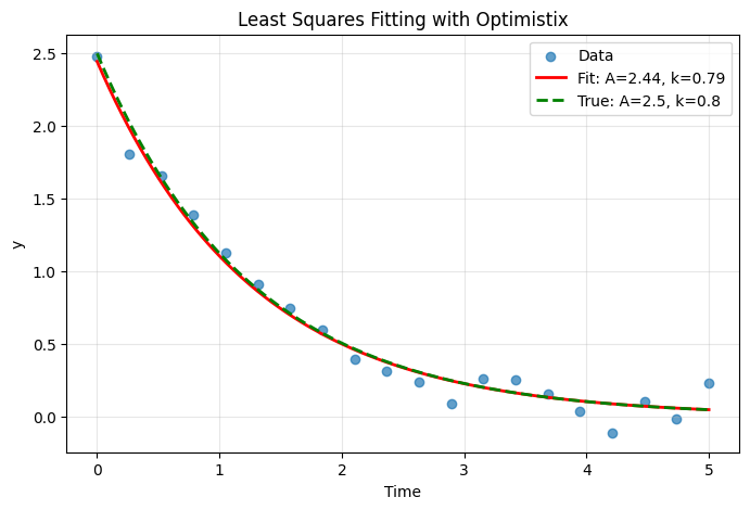
# Fit exponential decay: y = A * exp(-k * t)
# Generate synthetic data
t_data = jnp.linspace(0, 5, 20)
A_true, k_true = 2.5, 0.8
y_true = A_true * jnp.exp(-k_true * t_data)
noise = 0.1 * jax.random.normal(jax.random.PRNGKey(42), t_data.shape)
y_data = y_true + noise

def residuals(params, args):
    """Residuals for least squares fitting."""
    A, k = params
    t, y = args
    y_model = A * jnp.exp(-k * t)
    return y_model - y  # Vector of residuals

# Levenberg-Marquardt
solver = optx.LevenbergMarquardt(rtol=1e-8, atol=1e-8)
params0 = jnp.array([1.0, 0.5])  # Initial guess

solution = optx.least_squares(residuals, solver, params0, args=(t_data, y_data))

A_fit, k_fit = solution.value
print(f"Fitted parameters:")
print(f"  A = {A_fit:.4f} (true: {A_true})")
print(f"  k = {k_fit:.4f} (true: {k_true})")
Fitted parameters:
  A = 2.4444 (true: 2.5)
  k = 0.7945 (true: 0.8)
# Plot fit
t_fine = jnp.linspace(0, 5, 100)
y_fit = A_fit * jnp.exp(-k_fit * t_fine)

plt.figure(figsize=(8, 5))
plt.scatter(t_data, y_data, label='Data', alpha=0.7)
plt.plot(t_fine, y_fit, 'r-', label=f'Fit: A={A_fit:.2f}, k={k_fit:.2f}', linewidth=2)
plt.plot(t_fine, A_true * jnp.exp(-k_true * t_fine), 'g--',
         label=f'True: A={A_true}, k={k_true}', linewidth=2)
plt.xlabel('Time')
plt.ylabel('y')
plt.title('Least Squares Fitting with Optimistix')
plt.legend()
plt.grid(True, alpha=0.3)
plt.show()
6. Implicit Differentiation#
A key feature of optimistix is differentiating through the solver.
Given: \(x^* = \text{solve}(f, x_0, \theta)\) where \(\theta\) are parameters,
We can compute: \(\frac{dx^*}{d\theta}\) using the implicit function theorem.
# Example: How does the flash vapor fraction change with K-values?

def flash_calculation(K):
    """Solve flash calculation for given K-values.
    Returns vapor fraction V.
    """
    z = jnp.array([0.3, 0.4, 0.3])  # Fixed feed composition

    def residual(V, args):
        return jnp.sum(z * (K - 1) / (1 + V * (K - 1)))

    solver = optx.Newton(rtol=1e-10, atol=1e-10)
    V0 = jnp.array(0.5)
    solution = optx.root_find(residual, solver, V0)
    return solution.value

# K-values
K = jnp.array([3.0, 1.5, 0.5])

# Calculate V and its sensitivity to K
V = flash_calculation(K)
dV_dK = jax.jacobian(flash_calculation)(K)

print(f"Vapor fraction: V = {float(V):.6f}")
print(f"\nSensitivity dV/dK:")
for i, (Ki, dVi) in enumerate(zip(K, dV_dK)):
    print(f"  Component {i+1}: K = {Ki:.1f}, dV/dK = {dVi:.4f}")
Vapor fraction: V = 1.067639

Sensitivity dV/dK:
  Component 1: K = 3.0, dV/dK = 0.0599
  Component 2: K = 1.5, dV/dK = 0.3336
  Component 3: K = 0.5, dV/dK = 2.7084
# Verify sensitivity numerically
eps = 1e-6
dV_dK_numerical = []
for i in range(3):
    K_plus = K.at[i].add(eps)
    K_minus = K.at[i].add(-eps)
    dV = (flash_calculation(K_plus) - flash_calculation(K_minus)) / (2 * eps)
    dV_dK_numerical.append(float(dV))

print("Verification (numerical differentiation):")
print(f"  dV/dK (AD):        {dV_dK}")
print(f"  dV/dK (numerical): {jnp.array(dV_dK_numerical)}")
Verification (numerical differentiation):
  dV/dK (AD):        [0.05987755 0.33358499 2.70837418]
  dV/dK (numerical): [0.05987755 0.33358499 2.70837418]
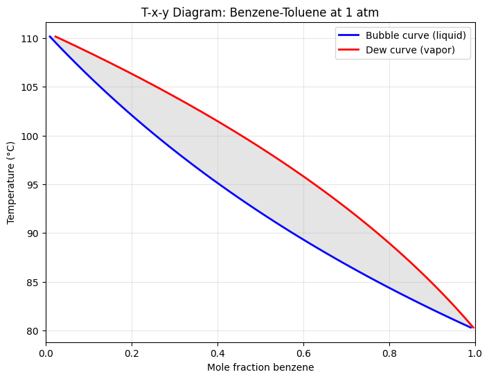
7. Chemical Engineering: VLE Calculation#
Solve bubble point calculation with Antoine equation.
# Antoine equation for vapor pressure
def antoine_pressure(T, A, B, C):
    """Antoine equation: log10(P) = A - B/(C + T)
    T in °C, P in mmHg
    """
    return 10**(A - B / (C + T))

# Antoine coefficients for benzene and toluene
# (A, B, C) with T in °C, P in mmHg
benzene = (6.90565, 1211.033, 220.790)
toluene = (6.95334, 1343.943, 219.377)

def bubble_point_residual(T, args):
    """Residual for bubble point: sum(y_i) - 1 = sum(x_i * P_i^sat / P) - 1
    """
    x, P_total = args  # Liquid composition, total pressure

    # Vapor pressures at temperature T
    P_benz = antoine_pressure(T, *benzene)
    P_tol = antoine_pressure(T, *toluene)
    P_sat = jnp.array([P_benz, P_tol])

    # Raoult's law: y_i = x_i * P_i^sat / P
    y = x * P_sat / P_total

    return jnp.sum(y) - 1.0

# Bubble point of 50/50 benzene/toluene at 760 mmHg
x = jnp.array([0.5, 0.5])
P_total = 760.0  # mmHg (1 atm)

solver = optx.Newton(rtol=1e-8, atol=1e-8)
T0 = jnp.array(90.0)  # Initial guess in °C

solution = optx.root_find(
    bubble_point_residual, solver, T0,
    args=(x, P_total)
)

T_bubble = float(solution.value)
print(f"Bubble point temperature: {T_bubble:.2f} °C")

# Calculate vapor composition
P_benz = antoine_pressure(T_bubble, *benzene)
P_tol = antoine_pressure(T_bubble, *toluene)
y = x * jnp.array([P_benz, P_tol]) / P_total

print(f"\nVapor composition:")
print(f"  Benzene: {float(y[0]):.4f}")
print(f"  Toluene: {float(y[1]):.4f}")
Bubble point temperature: 92.11 °C

Vapor composition:
  Benzene: 0.7136
  Toluene: 0.2864
# Generate T-x-y diagram using vmap
def bubble_point(x_benz):
    """Calculate bubble point for given benzene fraction."""
    x = jnp.array([x_benz, 1 - x_benz])

    solution = optx.root_find(
        bubble_point_residual,
        optx.Newton(rtol=1e-8, atol=1e-8),
        jnp.array(90.0),
        args=(x, 760.0)
    )

    T = solution.value
    P_benz = antoine_pressure(T, *benzene)
    y_benz = x_benz * P_benz / 760.0

    return T, y_benz

# Vectorize over compositions
x_range = jnp.linspace(0.01, 0.99, 50)
T_bubble_curve, y_curve = vmap(bubble_point)(x_range)

# Plot T-x-y diagram
plt.figure(figsize=(8, 6))
plt.plot(x_range, T_bubble_curve, 'b-', label='Bubble curve (liquid)', linewidth=2)
plt.plot(y_curve, T_bubble_curve, 'r-', label='Dew curve (vapor)', linewidth=2)
plt.fill_betweenx(T_bubble_curve, x_range, y_curve, alpha=0.2, color='gray')
plt.xlabel('Mole fraction benzene')
plt.ylabel('Temperature (°C)')
plt.title('T-x-y Diagram: Benzene-Toluene at 1 atm')
plt.legend()
plt.grid(True, alpha=0.3)
plt.xlim(0, 1)
plt.show()
8. Advanced: Custom Solvers and Options#
Optimistix allows fine-grained control over solver behavior.
# Custom Newton solver with damping
def difficult_function(x, args):
    """A function that's hard to solve without damping."""
    return jnp.array([
        x[0]**3 - 3*x[0]*x[1]**2 - 1,
        3*x[0]**2*x[1] - x[1]**3
    ])

# Standard Newton may diverge
# Use chord method or adjust settings
solver = optx.Newton(
    rtol=1e-8,
    atol=1e-8,
)

x0 = jnp.array([0.5, 0.5])

try:
    solution = optx.root_find(difficult_function, solver, x0, max_steps=100)
    print(f"Solution: {solution.value}")
    print(f"Residual: {jnp.linalg.norm(difficult_function(solution.value, None)):.2e}")
except Exception as e:
    print(f"Solver issue: {e}")
Solution: [-0.5        0.8660254]
Residual: 2.48e-16
# Use throw=False to handle non-convergence gracefully
def risky_solve(x0):
    solver = optx.Newton(rtol=1e-8, atol=1e-8)

    solution = optx.root_find(
        difficult_function,
        solver,
        x0,
        max_steps=50,
        throw=False  # Don't raise exception on failure
    )

    # Check result
    if solution.result == optx.RESULTS.successful:
        return solution.value, True
    else:
        return solution.value, False

# Try different starting points
starts = [jnp.array([0.5, 0.5]), jnp.array([1.0, 0.0]), jnp.array([2.0, 1.0])]

for x0 in starts:
    result, success = risky_solve(x0)
    status = "✓" if success else "✗"
    print(f"Start {x0}: {status} -> {result}")
Start [0.5 0.5]: ✓ -> [-0.5        0.8660254]
Start [1. 0.]: ✓ -> [1. 0.]
Start [2. 1.]: ✓ -> [ 1.00000000e+00 -1.02231372e-17]
9. Summary#
Key Optimistix Functions#
Function |
Purpose |
Signature |
|---|---|---|
|
Solve f(x) = 0 |
|
|
Solve x = g(x) |
|
|
Find argmin f(x) |
|
|
Minimize |
Solver Selection Guide#
Problem |
Recommended |
|---|---|
1D root finding |
|
Multivariate root finding |
|
Fixed-point iteration |
|
Minimization |
|
Least squares |
|
Key Features#
Implicit differentiation: Gradients through solver automatically
vmap compatible: Batch problems efficiently
JIT compilable: Full speed optimization
Composable: Works with diffrax, optax, equinox
Resources#
Documentation: https://docs.kidger.site/optimistix/
GitHub: patrick-kidger/optimistix