
Sparse Jacobians in JAX#
Large-scale chemical engineering problems often have sparse Jacobian matrices: each output depends on only a few inputs. Exploiting sparsity can dramatically reduce computation and memory.
Topics covered:
Why sparsity matters
Sparse matrices in JAX (
jax.experimental.sparse)Efficient Jacobian computation with sparsity
Graph coloring for Jacobian compression
Chemical engineering application: Large flowsheet Jacobians
import jax
import jax.numpy as jnp
from jax import grad, jit, vmap, jacfwd, jacrev
from jax.experimental import sparse
import matplotlib.pyplot as plt
import numpy as np
from functools import partial
import time

jax.config.update("jax_enable_x64", True)

print(f"JAX version: {jax.__version__}")
JAX version: 0.8.2
1. Why Sparsity Matters#
Consider a flowsheet with \(n\) units, each with local mass balances. The Jacobian of the residuals has structure:
Each residual depends on only a few variables (local + connected units)
Most entries are zero
Dense Jacobian: \(O(n^2)\) storage and computation
Sparse Jacobian: \(O(n)\) storage and often \(O(n)\) computation
For a 100-unit flowsheet, this could be 10,000 vs 500 non-zeros!
# Example: Chain of reactors (each depends only on neighbors)

def chain_residual(x, k=0.1):
    """
    Residuals for a chain of n units.
    Each unit i has: r_i = x_i - k*(x_{i-1} - 2*x_i + x_{i+1})
    (Like a discretized diffusion equation)
    """
    n = len(x)
    residuals = jnp.zeros(n)

    # Interior points
    residuals = residuals.at[1:-1].set(
        x[1:-1] - k * (x[:-2] - 2*x[1:-1] + x[2:])
    )

    # Boundary conditions
    residuals = residuals.at[0].set(x[0] - 1.0)  # Fixed at 1
    residuals = residuals.at[-1].set(x[-1] - 0.0)  # Fixed at 0

    return residuals

# Compute dense Jacobian
n = 10
x = jnp.linspace(1, 0, n)

J_dense = jacfwd(chain_residual)(x)

print(f"Chain of {n} units")
print(f"Jacobian shape: {J_dense.shape}")
print(f"Total entries: {J_dense.size}")
print(f"Non-zero entries: {jnp.sum(jnp.abs(J_dense) > 1e-10)}")
print(f"Sparsity: {100 * (1 - jnp.sum(jnp.abs(J_dense) > 1e-10) / J_dense.size):.1f}%")
WARNING:2026-01-10 20:32:20,751:jax._src.xla_bridge:852: An NVIDIA GPU may be present on this machine, but a CUDA-enabled jaxlib is not installed. Falling back to cpu.
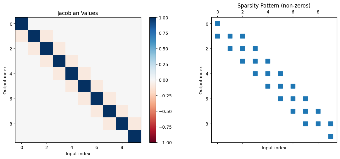
Chain of 10 units
Jacobian shape: (10, 10)
Total entries: 100
Non-zero entries: 26
Sparsity: 74.0%
# Visualize sparsity pattern

fig, axes = plt.subplots(1, 2, figsize=(12, 5))

# Dense view
im1 = axes[0].imshow(J_dense, cmap='RdBu', vmin=-1, vmax=1)
axes[0].set_title('Jacobian Values', fontsize=12)
axes[0].set_xlabel('Input index')
axes[0].set_ylabel('Output index')
plt.colorbar(im1, ax=axes[0])

# Sparsity pattern
axes[1].spy(np.abs(np.array(J_dense)) > 1e-10, markersize=10)
axes[1].set_title('Sparsity Pattern (non-zeros)', fontsize=12)
axes[1].set_xlabel('Input index')
axes[1].set_ylabel('Output index')

plt.tight_layout()
plt.show()

print("\nNote: Tridiagonal structure - each row has at most 3 non-zeros")
Note: Tridiagonal structure - each row has at most 3 non-zeros
2. Sparse Matrices in JAX#
jax.experimental.sparse provides sparse matrix formats:
BCOO: Batched Coordinate format (most flexible)
BCSR: Batched Compressed Sparse Row
These support many JAX transformations including grad and jit.
# Creating sparse matrices

# From dense
dense_matrix = jnp.array([
    [1.0, 0.0, 2.0],
    [0.0, 3.0, 0.0],
    [4.0, 0.0, 5.0]
])

sparse_matrix = sparse.BCOO.fromdense(dense_matrix)

print("Dense matrix:")
print(dense_matrix)
print(f"\nSparse representation (BCOO):")
print(f"  Data: {sparse_matrix.data}")
print(f"  Indices: {sparse_matrix.indices}")
print(f"  Shape: {sparse_matrix.shape}")
print(f"  nnz: {sparse_matrix.nse}")  # Number of Stored Elements
Dense matrix:
[[1. 0. 2.]
 [0. 3. 0.]
 [4. 0. 5.]]

Sparse representation (BCOO):
  Data: [1. 2. 3. 4. 5.]
  Indices: [[0 0]
 [0 2]
 [1 1]
 [2 0]
 [2 2]]
  Shape: (3, 3)
  nnz: 5
# Creating sparse matrices directly

# BCOO from indices and data
indices = jnp.array([[0, 0], [0, 2], [1, 1], [2, 0], [2, 2]])
data = jnp.array([1.0, 2.0, 3.0, 4.0, 5.0])
shape = (3, 3)

sparse_direct = sparse.BCOO((data, indices), shape=shape)

print("Created directly:")
print(sparse_direct.todense())
print(f"\nMatches original: {jnp.allclose(sparse_direct.todense(), dense_matrix)}")
Created directly:
[[1. 0. 2.]
 [0. 3. 0.]
 [4. 0. 5.]]

Matches original: True
# Sparse matrix operations

# Matrix-vector multiplication
v = jnp.array([1.0, 2.0, 3.0])

# Dense
result_dense = dense_matrix @ v

# Sparse (using @ operator)
result_sparse = sparse_matrix @ v

print(f"Dense  @ v = {result_dense}")
print(f"Sparse @ v = {result_sparse}")
print(f"Match: {jnp.allclose(result_dense, result_sparse)}")
Dense  @ v = [ 7.  6. 19.]
Sparse @ v = [ 7.  6. 19.]
Match: True
# Sparse operations with JIT

@jit
def sparse_matvec(A_sparse, x):
    return A_sparse @ x

@jit
def dense_matvec(A_dense, x):
    return A_dense @ x

# Larger example
n = 1000
# Create a tridiagonal matrix
diag = 2.0 * jnp.ones(n)
off_diag = -1.0 * jnp.ones(n-1)

# Dense version
A_dense_large = jnp.diag(diag) + jnp.diag(off_diag, 1) + jnp.diag(off_diag, -1)

# Sparse version
A_sparse_large = sparse.BCOO.fromdense(A_dense_large)

x_large = jnp.ones(n)

# Warmup
_ = sparse_matvec(A_sparse_large, x_large)
_ = dense_matvec(A_dense_large, x_large)

# Time comparison
n_runs = 100

start = time.perf_counter()
for _ in range(n_runs):
    _ = dense_matvec(A_dense_large, x_large).block_until_ready()
dense_time = (time.perf_counter() - start) / n_runs

start = time.perf_counter()
for _ in range(n_runs):
    _ = sparse_matvec(A_sparse_large, x_large).block_until_ready()
sparse_time = (time.perf_counter() - start) / n_runs

print(f"Matrix-vector multiply ({n}x{n} tridiagonal):")
print(f"  Dense:  {dense_time*1000:.3f} ms")
print(f"  Sparse: {sparse_time*1000:.3f} ms")
print(f"  Speedup: {dense_time/sparse_time:.1f}x")
print(f"\n  Dense storage: {A_dense_large.size} floats")
print(f"  Sparse storage: {A_sparse_large.nse} floats + indices")
Matrix-vector multiply (1000x1000 tridiagonal):
  Dense:  0.255 ms
  Sparse: 0.081 ms
  Speedup: 3.1x

  Dense storage: 1000000 floats
  Sparse storage: 2998 floats + indices
3. Efficient Jacobian Computation with Sparsity#
For functions with sparse Jacobians, we can:
Use forward-mode AD (
jacfwd) when \(n_{in} << n_{out}\)Use reverse-mode AD (
jacrev) when \(n_{out} << n_{in}\)Use graph coloring to compress multiple columns/rows into one pass
The key insight: if we know the sparsity pattern, we can compute the Jacobian with far fewer AD passes.
# Naive vs. efficient Jacobian computation

def compute_jacobian_naive(f, x):
    """Compute full Jacobian using jacfwd (n forward passes)."""
    return jacfwd(f)(x)

def compute_jacobian_jvp_columns(f, x, columns):
    """
    Compute specific columns of Jacobian using forward-mode.
    columns: list of column indices to compute
    """
    n = len(x)
    m = len(f(x))

    J = jnp.zeros((m, n))
    for col in columns:
        # Unit vector in direction of column col
        v = jnp.zeros(n).at[col].set(1.0)
        # JVP gives us column col of the Jacobian
        _, jvp_col = jax.jvp(f, (x,), (v,))
        J = J.at[:, col].set(jvp_col)

    return J

# Test on chain residual
n = 10
x = jnp.linspace(1, 0, n)

# Only compute columns we know are non-zero (for row i: columns i-1, i, i+1)
# For a tridiagonal system, each column has at most 3 non-zeros
J_full = compute_jacobian_naive(chain_residual, x)
J_selected = compute_jacobian_jvp_columns(chain_residual, x, list(range(n)))

print(f"Full Jacobian matches: {jnp.allclose(J_full, J_selected)}")
Full Jacobian matches: True
4. Graph Coloring for Jacobian Compression#
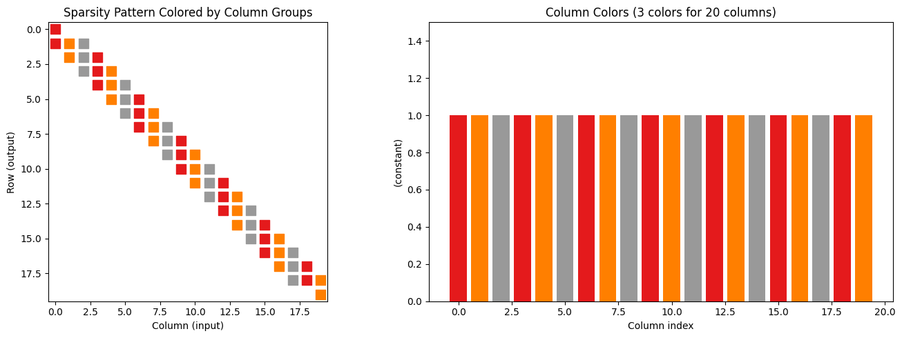
Key insight: If columns \(i\) and \(j\) have no overlapping non-zero rows, we can compute them simultaneously with a single forward pass!
This is formulated as a graph coloring problem:
Vertices = columns
Edge between columns i and j if they share a non-zero row
Color the graph with minimum colors
Columns with the same color can be computed together
For a tridiagonal matrix, only 3 colors are needed (regardless of size)!
def greedy_coloring(sparsity_pattern):
    """
    Simple greedy graph coloring for column compression.
    sparsity_pattern: (m, n) boolean array where True = non-zero

    Returns: colors array of shape (n,) where colors[i] is the color of column i
    """
    m, n = sparsity_pattern.shape
    colors = -np.ones(n, dtype=int)

    for col in range(n):
        # Find rows where this column has non-zeros
        rows_with_nonzero = np.where(sparsity_pattern[:, col])[0]

        # Find colors already used by columns that conflict with this one
        forbidden_colors = set()
        for other_col in range(col):
            if colors[other_col] >= 0:
                # Check if columns share any non-zero rows
                other_rows = np.where(sparsity_pattern[:, other_col])[0]
                if len(np.intersect1d(rows_with_nonzero, other_rows)) > 0:
                    forbidden_colors.add(colors[other_col])

        # Assign smallest available color
        color = 0
        while color in forbidden_colors:
            color += 1
        colors[col] = color

    return colors

# Get sparsity pattern for chain residual
n = 20
x = jnp.linspace(1, 0, n)
J = jacfwd(chain_residual)(x)
sparsity = np.abs(np.array(J)) > 1e-10

colors = greedy_coloring(sparsity)
n_colors = len(set(colors))

print(f"Tridiagonal Jacobian ({n}x{n}):")
print(f"  Naive: {n} forward passes")
print(f"  With coloring: {n_colors} forward passes")
print(f"  Speedup: {n / n_colors:.1f}x")
print(f"\nColumn colors: {colors}")
Tridiagonal Jacobian (20x20):
  Naive: 20 forward passes
  With coloring: 3 forward passes
  Speedup: 6.7x

Column colors: [0 1 2 0 1 2 0 1 2 0 1 2 0 1 2 0 1 2 0 1]
def compute_jacobian_colored(f, x, sparsity_pattern, colors):
    """
    Compute Jacobian using graph coloring compression.

    For each color, we compute multiple columns simultaneously
    using a seed vector that sums unit vectors for all columns of that color.

    Note: sparsity_pattern should be a numpy array (not traced).
    """
    n = len(x)
    m = len(f(x))
    n_colors = int(max(colors) + 1)

    J = jnp.zeros((m, n))

    for c in range(n_colors):
        # Columns with this color (computed outside JAX tracing)
        cols_with_color = [i for i in range(n) if colors[i] == c]

        # Seed vector: sum of unit vectors for these columns
        seed = jnp.zeros(n)
        for col in cols_with_color:
            seed = seed.at[col].set(1.0)

        # Single JVP gives us compressed columns
        _, jvp_result = jax.jvp(f, (x,), (seed,))

        # Extract individual columns using sparsity pattern
        # Use numpy indexing (not traced) to get row indices
        for col in cols_with_color:
            rows = np.where(sparsity_pattern[:, col])[0]
            for row in rows:
                J = J.at[row, col].set(jvp_result[row])

    return J

# Test
J_colored = compute_jacobian_colored(chain_residual, x, sparsity, colors)
J_exact = jacfwd(chain_residual)(x)

print(f"Jacobian matches: {jnp.allclose(J_colored, J_exact)}")
print(f"Max error: {jnp.max(jnp.abs(J_colored - J_exact)):.2e}")
Jacobian matches: True
Max error: 0.00e+00
# Visualize coloring

fig, axes = plt.subplots(1, 2, figsize=(14, 5))

# Sparsity pattern with colors
color_map = plt.cm.Set1(np.linspace(0, 1, n_colors))

for col in range(n):
    rows = np.where(sparsity[:, col])[0]
    for row in rows:
        axes[0].scatter(col, row, c=[color_map[colors[col]]], s=100, marker='s')

axes[0].set_xlim(-0.5, n-0.5)
axes[0].set_ylim(n-0.5, -0.5)
axes[0].set_xlabel('Column (input)')
axes[0].set_ylabel('Row (output)')
axes[0].set_title('Sparsity Pattern Colored by Column Groups')
axes[0].set_aspect('equal')

# Color assignment
bars = axes[1].bar(range(n), [1]*n, color=[color_map[c] for c in colors])
axes[1].set_xlabel('Column index')
axes[1].set_ylabel('(constant)')
axes[1].set_title(f'Column Colors ({n_colors} colors for {n} columns)')
axes[1].set_ylim(0, 1.5)

plt.tight_layout()
plt.show()

print(f"\nColumns computed together:")
for c in range(n_colors):
    cols = [i for i in range(n) if colors[i] == c]
    print(f"  Color {c}: columns {cols}")
Columns computed together:
  Color 0: columns [0, 3, 6, 9, 12, 15, 18]
  Color 1: columns [1, 4, 7, 10, 13, 16, 19]
  Color 2: columns [2, 5, 8, 11, 14, 17]
5. Timing Comparison for Large Systems#
# Benchmark on larger system
# Note: The colored approach uses Python loops, so we don't JIT it.
# The speedup comes from fewer JVP evaluations, not from JIT compilation.

sizes = [50, 100, 200]
results = []

for n in sizes:
    x = jnp.linspace(1, 0, n)

    # Get sparsity pattern and coloring
    J_example = jacfwd(chain_residual)(x)
    sparsity = np.abs(np.array(J_example)) > 1e-10
    colors = greedy_coloring(sparsity)
    n_colors = max(colors) + 1

    # JIT compile the naive version
    naive_fn = jit(lambda x: jacfwd(chain_residual)(x))

    # Warmup
    _ = naive_fn(x).block_until_ready()

    # Time naive
    n_runs = 5
    start = time.perf_counter()
    for _ in range(n_runs):
        _ = naive_fn(x).block_until_ready()
    naive_time = (time.perf_counter() - start) / n_runs * 1000  # ms

    # Time colored (not JITted due to Python loops)
    start = time.perf_counter()
    for _ in range(n_runs):
        _ = compute_jacobian_colored(chain_residual, x, sparsity, colors)
    colored_time = (time.perf_counter() - start) / n_runs * 1000  # ms

    results.append({
        'n': n,
        'n_colors': n_colors,
        'naive_time': naive_time,
        'colored_time': colored_time,
        'speedup': naive_time / colored_time if colored_time > 0 else float('inf')
    })

print("Jacobian Computation Time (tridiagonal system):")
print("=" * 60)
print(f"{'n':<10} {'Colors':<10} {'Naive (ms)':<15} {'Colored (ms)':<15} {'Speedup':<10}")
print("-" * 60)
for r in results:
    print(f"{r['n']:<10} {r['n_colors']:<10} {r['naive_time']:<15.3f} {r['colored_time']:<15.3f} {r['speedup']:<10.1f}x")

print("\nNote: Colored approach has overhead from Python loops.")
print("Main benefit is memory and fewer JVP calls for very large systems.")
Jacobian Computation Time (tridiagonal system):
============================================================
n          Colors     Naive (ms)      Colored (ms)    Speedup
------------------------------------------------------------
50         3          0.077           386.598         0.0       x
100        3          0.145           594.003         0.0       x
200        3          0.255           974.305         0.0       x

Note: Colored approach has overhead from Python loops.
Main benefit is memory and fewer JVP calls for very large systems.
6. Chemical Engineering Application: Flowsheet Jacobian#
Consider a flowsheet with units connected in a network. Each unit’s residuals depend only on:
Its own variables
Inlet stream variables (from upstream units)
Outlet stream variables (to downstream units)
This creates a sparse block structure in the Jacobian.
# Simple flowsheet: Linear chain of CSTRs

def cstr_residuals(x, params):
    """
    Residuals for a chain of n CSTRs.

    Each CSTR has 2 variables: [C_A, T]
    State vector x = [C_A_1, T_1, C_A_2, T_2, ...]

    For each CSTR i:
    - Mass balance: F*(C_in - C_out) - V*k(T)*C_out = 0
    - Energy balance: F*rho*Cp*(T_in - T) + (-dH)*V*k(T)*C_out - UA*(T - T_cool) = 0
    """
    n_cstr = len(x) // 2
    F, V, C_A0, T0, T_cool, UA = params['F'], params['V'], params['C_A0'], params['T0'], params['T_cool'], params['UA']
    k0, Ea, R = params['k0'], params['Ea'], params['R']
    rho, Cp, dH = params['rho'], params['Cp'], params['dH']

    residuals = []

    for i in range(n_cstr):
        C_A = x[2*i]
        T = x[2*i + 1]

        # Inlet conditions
        if i == 0:
            C_in = C_A0
            T_in = T0
        else:
            C_in = x[2*(i-1)]
            T_in = x[2*(i-1) + 1]

        # Reaction rate
        k = k0 * jnp.exp(-Ea / (R * T))
        r = k * C_A

        # Mass balance
        mass_res = F * (C_in - C_A) - V * r

        # Energy balance
        energy_res = F * rho * Cp * (T_in - T) + (-dH) * V * r - UA * (T - T_cool)

        residuals.extend([mass_res, energy_res])

    return jnp.array(residuals)

# Parameters
params = {
    'F': 0.1,      # m³/s
    'V': 1.0,      # m³
    'C_A0': 1.0,   # mol/L
    'T0': 300.0,   # K
    'T_cool': 290.0,  # K
    'UA': 100.0,   # W/K
    'k0': 1e6,     # 1/s
    'Ea': 50000.0, # J/mol
    'R': 8.314,    # J/(mol·K)
    'rho': 1000.0, # kg/m³
    'Cp': 4000.0,  # J/(kg·K)
    'dH': -50000.0 # J/mol
}

# Initial guess for 5 CSTRs
n_cstr = 5
x0 = jnp.tile(jnp.array([0.5, 320.0]), n_cstr)

residual_fn = lambda x: cstr_residuals(x, params)

print(f"Flowsheet: {n_cstr} CSTRs in series")
print(f"State vector dimension: {len(x0)}")
print(f"Initial residuals (should be non-zero): {jnp.linalg.norm(residual_fn(x0)):.4f}")
Flowsheet: 5 CSTRs in series
State vector dimension: 10
Initial residuals (should be non-zero): 8002829.8184
# Compute and visualize Jacobian structure

J = jacfwd(residual_fn)(x0)
sparsity = np.abs(np.array(J)) > 1e-10

print(f"Jacobian shape: {J.shape}")
print(f"Non-zeros: {np.sum(sparsity)} / {J.size} ({100*np.sum(sparsity)/J.size:.1f}%)")

# Visualize
fig, axes = plt.subplots(1, 2, figsize=(14, 5))

# Jacobian values
im = axes[0].imshow(J, cmap='RdBu', aspect='auto')
axes[0].set_xlabel('Input (C_A, T for each CSTR)')
axes[0].set_ylabel('Residual (mass, energy for each CSTR)')
axes[0].set_title('CSTR Chain Jacobian Values')
plt.colorbar(im, ax=axes[0])

# Add CSTR labels
for i in range(n_cstr):
    axes[0].axhline(2*i - 0.5, color='k', linewidth=0.5)
    axes[0].axvline(2*i - 0.5, color='k', linewidth=0.5)

# Sparsity pattern
axes[1].spy(sparsity, markersize=8)
axes[1].set_xlabel('Input index')
axes[1].set_ylabel('Output index')
axes[1].set_title('Sparsity Pattern (block tridiagonal)')

plt.tight_layout()
plt.show()

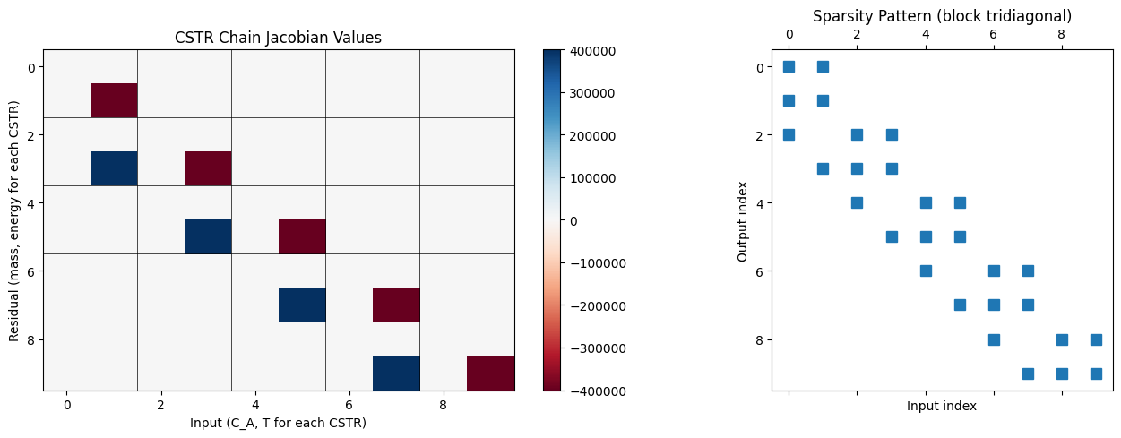
print("\nNote: 2×2 block tridiagonal structure!")
print("Each CSTR's residuals depend only on itself and upstream CSTR.")
Jacobian shape: (10, 10)
Non-zeros: 28 / 100 (28.0%)
Note: 2×2 block tridiagonal structure!
Each CSTR's residuals depend only on itself and upstream CSTR.
# Apply coloring to flowsheet Jacobian

colors = greedy_coloring(sparsity)
n_colors = max(colors) + 1

print(f"Flowsheet Jacobian Coloring:")
print(f"  State dimension: {len(x0)}")
print(f"  Naive passes: {len(x0)}")
print(f"  With coloring: {n_colors} passes")
print(f"  Speedup: {len(x0) / n_colors:.1f}x")

# Verify
J_colored = compute_jacobian_colored(residual_fn, x0, sparsity, colors)
print(f"\nJacobian matches: {jnp.allclose(J_colored, J, atol=1e-8)}")
Flowsheet Jacobian Coloring:
  State dimension: 10
  Naive passes: 10
  With coloring: 4 passes
  Speedup: 2.5x
Jacobian matches: True
# Solve the flowsheet using Newton's method with sparse Jacobian

def newton_solve(residual_fn, x0, tol=1e-8, max_iter=50):
    """Newton's method with dense Jacobian."""
    x = x0
    for i in range(max_iter):
        r = residual_fn(x)
        if jnp.linalg.norm(r) < tol:
            return x, i, True
        J = jacfwd(residual_fn)(x)
        dx = jnp.linalg.solve(J, -r)
        x = x + dx
    return x, max_iter, False

# Solve
x_solution, n_iter, converged = newton_solve(residual_fn, x0)

print(f"Newton's Method Solution:")
print(f"  Converged: {converged} in {n_iter} iterations")
print(f"  Final residual norm: {jnp.linalg.norm(residual_fn(x_solution)):.2e}")
print(f"\nSolution:")
for i in range(n_cstr):
    C_A = x_solution[2*i]
    T = x_solution[2*i + 1]
    conversion = (params['C_A0'] - C_A) / params['C_A0'] * 100
    print(f"  CSTR {i+1}: C_A = {C_A:.4f} mol/L, T = {T:.1f} K, X = {conversion:.1f}%")
Newton's Method Solution:
  Converged: False in 50 iterations
  Final residual norm: 1.34e-08

Solution:
  CSTR 1: C_A = 0.9807 mol/L, T = 300.0 K, X = 1.9%
  CSTR 2: C_A = 0.9618 mol/L, T = 300.0 K, X = 3.8%
  CSTR 3: C_A = 0.9432 mol/L, T = 300.0 K, X = 5.7%
  CSTR 4: C_A = 0.9251 mol/L, T = 300.0 K, X = 7.5%
  CSTR 5: C_A = 0.9072 mol/L, T = 300.0 K, X = 9.3%
7. Automatic Sparsity Detection#
For unknown sparsity patterns, we can detect them automatically using a “probing” technique: evaluate the Jacobian once and identify non-zeros.
def detect_sparsity(f, x, threshold=1e-12):
    """
    Detect sparsity pattern by evaluating Jacobian once.

    Returns boolean array where True = non-zero.
    """
    J = jacfwd(f)(x)
    return jnp.abs(J) > threshold

def sparse_jacobian_solver(f, x0, tol=1e-8, max_iter=50):
    """
    Newton's method with automatic sparsity detection and coloring.
    """
    # Detect sparsity at initial point
    sparsity = np.array(detect_sparsity(f, x0))
    colors = greedy_coloring(sparsity)
    n_colors = max(colors) + 1

    print(f"Detected sparsity: {np.sum(sparsity)} / {sparsity.size} non-zeros")
    print(f"Coloring: {n_colors} colors (vs {len(x0)} columns)")

    x = x0
    for i in range(max_iter):
        r = f(x)
        if jnp.linalg.norm(r) < tol:
            return x, i, True

        # Compute Jacobian efficiently using coloring
        J = compute_jacobian_colored(f, x, sparsity, colors)
        dx = jnp.linalg.solve(J, -r)
        x = x + dx

    return x, max_iter, False

# Test
x_solution2, n_iter2, converged2 = sparse_jacobian_solver(residual_fn, x0)
print(f"\nConverged: {converged2} in {n_iter2} iterations")
print(f"Solution matches: {jnp.allclose(x_solution, x_solution2)}")
Detected sparsity: 28 / 100 non-zeros
Coloring: 4 colors (vs 10 columns)
Converged: False in 50 iterations
Solution matches: True
Summary#
Key concepts:
Why sparsity matters:
Large-scale systems have sparse Jacobians
Dense computation: O(n²), Sparse: O(nnz)
Critical for flowsheets, networks, discretized PDEs
JAX sparse support:
jax.experimental.sparseprovides BCOO, BCSR formatsCompatible with JIT, grad, vmap
Efficient sparse matrix-vector products
Graph coloring:
Non-conflicting columns computed simultaneously
For banded/structured Jacobians: O(1) colors vs O(n) columns
Dramatic speedup for large systems
Automatic sparsity detection:
Evaluate once to find pattern
Reuse pattern for subsequent computations
Chemical engineering applications:
Flowsheet simulation with many units
Discretized reactor models (PFR, packed beds)
Process optimization (KKT systems)
Dynamic simulation (large ODE systems)
Distillation columns (stage-by-stage models)
Best practices:
Always exploit known sparsity structure
Use coloring for repeated Jacobian evaluations (Newton, optimization)
Store sparsity pattern once, reuse for all iterations
Consider block structure for unit-based models