Data Reconciliation of a Gas Transmission Network

Plant measurements disagree with the model. Meters drift, nominations do not close, and a pressure drop rarely matches the flow that supposedly caused it. Data reconciliation finds the smallest statistically weighted adjustment that makes the measurements satisfy the model equations:

\[\min_x \; (x - y)^T W (x - y) \quad \text{subject to} \quad F(x, \theta) = 0\]

The payoff is not just consistency. Because the model equations carry information the sensors do not, the reconciled estimates are more precise than the measurements — on the network below, by 58% to 93% in variance.

Everything reconciliation needs is derivative information: the constraint Jacobian \(A = \partial F/\partial x\), the covariance of the estimates, the sensitivity of each estimate to each measurement. A conventional flowsheet package hand-derives it unit by unit. Here jax.jacobian supplies it, which is what makes the same code work for a gas network, a reactor train, or an equation set you write on the spot.

What this notebook covers

2. The network and its true state

3. Corrupting it, and seeing the model reject the data

4. Reconciliation, and the precision it buys

5. Covariance two ways: the textbook formula and autodiff

6. Finding a biased flow meter

7. Estimating an unmeasured pipe fouling factor

8. The observability boundary — and what the compressor has to do with it

9. Sensor placement

(Section 1 is imports and plotting setup.)

1. Setup

import jax
import jax.numpy as jnp

jax.config.update("jax_enable_x64", True)

import numpy as np
import matplotlib.pyplot as plt
import difflow_gas as dg
from difflow_gas import verify
from difflow.reconciliation import (
    global_test,
    measurement_test,
    measurement_sensitivity,
    reconciled_covariance,
    sensor_ranking,
    serial_elimination,
    solve_reconciliation,
    ReconciliationStructureError,
)

# palette: categorical slots 1-2, plus the reserved "critical" status step
BLUE, ORANGE, RED, GREY = "#2a78d6", "#eb6834", "#d03b3b", "#8a8985"
INK, INK_SOFT, GRID = "#0b0b0b", "#52514e", "#eceae6"

def tidy(ax, axis="y"):
    """Recessive axes and grid, so the data carries the emphasis."""
    ax.spines[["top", "right"]].set_visible(False)
    for s in ax.spines.values():
        s.set_color("#d5d4d0")
    ax.tick_params(colors=INK_SOFT, labelsize=8, length=3)
    ax.grid(axis=axis, color=GRID, linewidth=0.8)
    ax.set_axisbelow(True)

print("JAX version:", jax.__version__)

JAX version: 0.11.0

2. The network

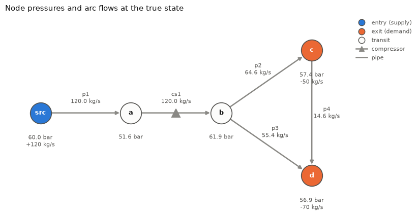
Five nodes, one compressor station, and a loop. Gas enters at src at 120 kg/s, is boosted by station cs1, and leaves at c (50 kg/s) and d (70 kg/s). Arcs p2, p3 and p4 form the loop b-c-d-b, which is what creates redundancy: the flow split around a loop is determined by the pipe resistances, so measuring it over-determines the state.

This is the network of 20_gas_network_flowsheets.ipynb, with realistic Weymouth coefficients for 0.6 m pipes at transmission scale.

RATIOS = {"cs1": 1.2}          # compressor pressure ratio
P_SLACK_PA = 60.0e5           # slack pressure at src (60 bar)

net = dg.GasNetwork(
    arcs={
        "p1":  ("src", "a", "pipe"),
        "cs1": ("a",   "b", "compressor"),
        "p2":  ("b",   "c", "pipe"),
        "p3":  ("b",   "d", "pipe"),
        "p4":  ("c",   "d", "pipe"),        # closes the loop b-c-d-b
    },
    beta={
        aid: dg.weymouth_beta(length_m=L, diameter_m=0.6, roughness_m=1e-4)
        for aid, L in [("p1", 20e3), ("p2", 40e3), ("p3", 60e3), ("p4", 80e3)]
    },
    supply_kg_s={"src": 120.0, "c": -50.0, "d": -70.0},
    pressure_bounds_bar={n: (30.0, 80.0) for n in ["src", "a", "b", "c", "d"]},
)

print(f"{len(net.nodes)} nodes, {len(net.arcs)} arcs, cycle rank {net.cycle_rank}")

5 nodes, 5 arcs, cycle rank 1

Solve it sequentially to get the true state that the measurements will be sampled around.

fs, dec = dg.build_network_flowsheet(
    net, root="src", p_slack_pa=P_SLACK_PA, ratios=RATIOS
)
streams = fs.solve(tol=1e-12, max_iter=500)

p_true = verify.node_pressures_bar(streams, dec)
q_true = verify.arc_flows_kg_s(streams, dec)

print("pressures (bar):", {k: round(v, 3) for k, v in p_true.items()})
print("flows (kg/s)   :", {k: round(v, 3) for k, v in q_true.items()})
print("all equations satisfied:", verify.residual_report(streams, net, dec).ok)

pressures (bar): {'src': 60.0, 'a': 51.624, 'b': 61.948, 'c': 57.406, 'd': 56.921}
flows (kg/s)   : {'p1': 120.0, 'cs1': 120.0, 'p2': 64.612, 'p3': 55.388, 'p4': 14.612}
all equations satisfied: True

POS = {"src": (0, 0), "a": (1.15, 0), "b": (2.3, 0),
       "c": (3.45, 0.8), "d": (3.45, -0.8)}

fig, ax = plt.subplots(figsize=(8.5, 4.4))
dg.draw_network(
    net, ax=ax, pos=POS, pressures=p_true, flows=q_true,
    title="Node pressures and arc flows at the true state",
)
plt.tight_layout()
plt.show()

The state vector

gas_state_layout packs pressures (bar), signed arc flows (kg/s) and boundary flows into one vector. The boundary flows being variables rather than fixed parameters matters more than it looks: with them held fixed, the node-balance block of the Jacobian is the network’s incidence matrix, whose rank is only \(n_{\text{nodes}} - 1\), and the KKT system below would be singular for purely structural reasons. Carrying them as unknowns gives every balance row a \(+1\) in its own column.

It also reflects reality. Real nominations do not sum to zero — and GasNetwork refuses to store supplies that do not. So the measured nominations live in the measurement vector, and making them close is precisely the reconciliation’s job.

layout = dg.gas_state_layout(net)
residual_fn = dg.network_residual_fn(net, layout, ratios=RATIOS)

x_true = layout.pack(p_true, q_true, net.supply_kg_s)

print(f"{layout.size} variables:", layout.names)
print(f"\n{len(dg.residual_names(net, layout))} equations:", dg.residual_names(net, layout))
print("\nF(x_true) max residual:", float(jnp.max(jnp.abs(residual_fn(x_true)))))

13 variables: ['p_a', 'p_b', 'p_c', 'p_d', 'p_src', 'q_cs1', 'q_p1', 'q_p2', 'q_p3', 'q_p4', 's_c', 's_d', 's_src']

10 equations: ['balance_a', 'balance_b', 'balance_c', 'balance_d', 'balance_src', 'resistance_p1', 'resistance_p2', 'resistance_p3', 'resistance_p4', 'compressor_cs1']

F(x_true) max residual: 1.2986518527213775e-09

Note the last equation. difflow_gas.verify deliberately omits the compressor relation \(p_{\text{to}} = r\,p_{\text{from}}\), because a sequential solve satisfies it by construction — there is nothing to check. A reconciliation formulation cannot omit it: without that row the pressures downstream of the station are untied from the ones upstream. Section 8 shows it is exactly what makes the loop observable.

3. Corrupting the data

Real transmission practice: pressure transmitters are good, flow meters less so, and nominated boundary flows are the least reliable numbers in the system.

sigma = dg.measurement_sigma(
    layout,
    sigma_p_bar=0.3,          # pressure transmitters
    sigma_q_kg_s=1.0,         # flow meters
    sigma_supply_kg_s=1.5,    # nominations
)
y = dg.perturb(x_true, sigma, jax.random.PRNGKey(0))

measured_p = {n: float(y[layout.index(f"p_{n}")]) for n in layout.nodes}
measured_q = {a: float(y[layout.index(f"q_{a}")]) for a in layout.arcs}
before = verify.residuals_from_values(measured_p, measured_q, net)

print(f"worst node imbalance   : {before.max_node_imbalance_kg_s:8.4f} kg/s")
print(f"worst resistance error : {before.max_resistance_residual_bar2:8.4f} bar^2")
nomination_sum = sum(float(y[layout.index(f"s_{n}")]) for n in layout.supply_nodes)
print(f"\nnominations sum to     : {nomination_sum:8.4f} kg/s  (should be 0)")

worst node imbalance   :   1.5623 kg/s
worst resistance error :  97.6610 bar^2

nominations sum to     :  -0.2062 kg/s  (should be 0)

The raw measurements are physically impossible: gas appears and disappears at nodes, and the pipe laws are off by nearly 100 bar². Every number is individually plausible; collectively they are not.

4. Reconciliation

One call. sigma sets the weights, and the returned object carries the reconciled state, its covariance, and the observability structure.

res = dg.reconcile_network(net, y, sigma, layout, ratios=RATIOS)
print(res.summary())

objective 8.753 on 10 degrees of redundancy, |F| = 4.55e-13, converged = True

variable                 measured   reconciled     adjust     sigma    sd_hat
----------------------------------------------------------------------------
p_a                       51.5620      51.6985     0.1365    0.3000    0.1174
p_b                       61.7130      62.0382     0.3252    0.3000    0.1409
p_c                       57.9511      57.4973    -0.4538    0.3000    0.1565
p_d                       56.9776      56.9743    -0.0033    0.3000    0.1585
p_src                     60.0243      60.1001     0.0758    0.3000    0.1266
q_cs1                    119.6279     120.2752     0.6473    1.0000    0.5348
q_p1                     121.1902     120.2752    -0.9150    1.0000    0.5348
q_p2                      64.9507      64.6521    -0.2986    1.0000    0.3254
q_p3                      55.4728      55.6231     0.1503    1.0000    0.2718
q_p4                      13.7402      15.1823     1.4421    1.0000    0.6456
s_c                      -48.4182     -49.4697    -1.0515    1.5000    0.8258
s_d                      -72.3392     -70.8054     1.5338    1.5000    0.8190
s_src                    120.5513     120.2752    -0.2761    1.5000    0.5348

p_rec, q_rec, s_rec = dg.reconciled_values(res, layout)
# Check against the RECONCILED nominations: `net` carries the nominal ones,
# which the reconciliation was free to adjust.
net_rec = dg.GasNetwork(arcs=net.arcs, beta=net.beta, supply_kg_s=s_rec)
after = verify.residuals_from_values(p_rec, q_rec, net_rec)

print(f"worst resistance error : {after.max_resistance_residual_bar2:.3e} bar^2"
      f"   (was {before.max_resistance_residual_bar2:.4f})")
print(f"worst node imbalance   : {after.max_node_imbalance_kg_s:.3e} kg/s")
print(f"nominations sum to     : {sum(s_rec.values()):.3e} kg/s")
print(f"\nplugin's own verifier says consistent: {after.ok}")

worst resistance error : 1.298e-09 bar^2   (was 97.6610)
worst node imbalance   : 1.421e-14 kg/s
nominations sum to     : 1.421e-14 kg/s

plugin's own verifier says consistent: True

What the constraints bought

The reconciled standard deviations come from \(\Sigma_{\hat x} = [K^{-1}]_{11}\), the leading block of the inverse KKT matrix. Every estimate is sharper than its measurement. Some of the gain is plain replication — q_p1, q_cs1 and s_src all meter the same 120 kg/s, and the balances make them one number — but the loop variables improve only because the pipe laws and the compressor relation tie them together.

print(f"{'variable':<10} {'sigma':>8} {'sd_hat':>8} {'variance reduction':>20}")
print("-" * 50)
for i, name in enumerate(layout.names):
    s0, s1 = float(sigma[i]), res.std[name]
    print(f"{name:<10} {s0:8.3f} {s1:8.4f} {100 * (1 - (s1 / s0) ** 2):17.1f} %")

variable      sigma   sd_hat   variance reduction
--------------------------------------------------
p_a           0.300   0.1174              84.7 %
p_b           0.300   0.1409              77.9 %
p_c           0.300   0.1565              72.8 %
p_d           0.300   0.1585              72.1 %
p_src         0.300   0.1266              82.2 %
q_cs1         1.000   0.5348              71.4 %
q_p1          1.000   0.5348              71.4 %
q_p2          1.000   0.3254              89.4 %
q_p3          1.000   0.2718              92.6 %
q_p4          1.000   0.6456              58.3 %
s_c           1.500   0.8258              69.7 %
s_d           1.500   0.8190              70.2 %
s_src         1.500   0.5348              87.3 %

The same two facts as pictures — the adjustments on the left, and what they bought on the right. Adjustments are shown in units of each sensor’s own \(\sigma\) so that pressures, flows and nominations are comparable on one axis.

names = list(layout.names)
ypos = np.arange(len(names))[::-1]
adj_sigma = np.asarray(res.adjustment) / np.asarray(sigma)   # in sigma units
sd_ratio = np.array([res.std[n] for n in names]) / np.asarray(sigma)

fig, axes = plt.subplots(1, 2, figsize=(11.5, 4.6), sharey=True)

ax = axes[0]
ax.barh(ypos, adj_sigma, height=0.62,
        color=[BLUE if v < 0 else RED for v in adj_sigma], edgecolor="none")
ax.axvline(0, color=INK_SOFT, linewidth=1)
ax.set_yticks(ypos)
ax.set_yticklabels(names, fontsize=8)
ax.set_xlabel("adjustment  (multiples of the sensor's own $\\sigma$)",
              fontsize=9, color=INK_SOFT)
ax.set_title("How far each measurement had to move", fontsize=10, color=INK, loc="left")
for yy, v in zip(ypos, adj_sigma):
    ax.text(v + (0.05 if v >= 0 else -0.05), yy, f"{v:+.2f}", va="center",
            ha="left" if v >= 0 else "right", fontsize=7.5, color=INK_SOFT)
ax.set_xlim(min(adj_sigma.min() * 1.35, -0.6), max(adj_sigma.max() * 1.35, 0.6))
tidy(ax, axis="x")
ax.tick_params(axis="y", length=0)

ax = axes[1]
ax.hlines(ypos, sd_ratio, 1.0, color="#d5d4d0", linewidth=2, zorder=1)
ax.scatter(np.ones_like(sd_ratio), ypos, s=42, color=ORANGE, zorder=2,
           label="measurement $\\sigma$")
ax.scatter(sd_ratio, ypos, s=42, color=BLUE, zorder=3, label="after reconciliation")
ax.set_xlim(0, 1.18)
ax.set_xlabel("standard deviation, relative to the meter's own",
              fontsize=9, color=INK_SOFT)
ax.set_title("Precision the model equations buy", fontsize=10, color=INK, loc="left")
ax.legend(frameon=False, fontsize=8, loc="lower right",
          bbox_to_anchor=(1.0, 1.005), ncol=2, labelcolor=INK_SOFT)
for yy, v in zip(ypos, sd_ratio):
    ax.text(v - 0.03, yy, f"{100 * (1 - v ** 2):.0f}%", va="center", ha="right",
            fontsize=7.5, color=INK_SOFT)
tidy(ax, axis="x")
ax.tick_params(axis="y", length=0)

plt.tight_layout()
plt.show()

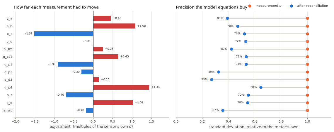
q_p4 gains the least. It is the loop’s longest leg (80 km) and carries only ~15 kg/s, so the balances constrain it least — which makes it the hardest place to catch a bad meter.

The degrees of redundancy are the number of independent checks the data must pass:

st = res.structure
print(f"equations                : {st.n_equations}")
print(f"measured / unmeasured    : {st.n_measured} / {st.n_unmeasured}")
print(f"degrees of redundancy    : {st.degree_of_redundancy}")
print(f"solvable                 : {st.solvable}")
print()
print(global_test(res))

equations                : 10
measured / unmeasured    : 13 / 0
degrees of redundancy    : 10
solvable                 : True

global test: chi2 = 8.753 on 10 dof, critical = 18.307, p = 0.556 -> no gross error

5. Covariance, two ways

The classical result says the reconciled covariance is a projection, \(\Sigma_{\hat x} = \Sigma - \Sigma A^T (A\Sigma A^T)^{-1} A \Sigma\).

But reconciliation is also just a function \(\hat x(y)\), so its covariance ought to follow from propagating \(\Sigma\) through the sensitivity \(S = \partial \hat x / \partial y\) — which jax.jacfwd can take straight through the solver. Do the two agree?

S = measurement_sensitivity(
    residual_fn, y, sigma, x0=x_true, scaling=res.scaling
)
Sigma = np.diag(np.asarray(sigma) ** 2)

autodiff_cov = np.asarray(S) @ Sigma @ np.asarray(S).T
formula_cov = np.asarray(res.covariance)

print("max |S Sigma S^T  -  Sigma_xhat| :", np.max(np.abs(autodiff_cov - formula_cov)))
print("largest covariance entry         :", np.max(np.abs(formula_cov)))
print("max |lambda| (constraint forces) :", float(jnp.max(jnp.abs(res.multipliers))))

max |S Sigma S^T  -  Sigma_xhat| : 0.009617096676138526
largest covariance entry         : 0.6818793838206372
max |lambda| (constraint forces) : 1.8680644638109334

Close, but not equal — and the reason is worth understanding.

For linear constraints the two are the same matrix identically: \(S = \Sigma_{\hat x} W\) and \(W \Sigma W = W\), so \(S \Sigma S^T = \Sigma_{\hat x}\) exactly. For nonlinear constraints they differ by the curvature term \(\sum_k \lambda_k \nabla^2 F_k\), which the covariance formula drops and differentiating the solver does not.

The gap is therefore proportional to the Lagrange multipliers — to how hard the constraints had to pull. On consistent data it vanishes:

print(f"{'noise level':>12} {'max |lambda|':>14} {'max |difference|':>18}")
print("-" * 46)
for scale in [0.0, 0.05, 0.2, 1.0, 3.0]:
    y_s = x_true + scale * (y - x_true)
    r_s = dg.reconcile_network(net, y_s, sigma, layout, ratios=RATIOS)
    S_s = measurement_sensitivity(
        residual_fn, y_s, sigma, x0=x_true, scaling=r_s.scaling
    )
    gap = np.max(np.abs(np.asarray(S_s) @ Sigma @ np.asarray(S_s).T
                        - np.asarray(r_s.covariance)))
    print(f"{scale:12.2f} {float(jnp.max(jnp.abs(r_s.multipliers))):14.4g} {gap:18.4g}")

 noise level   max |lambda|   max |difference|
----------------------------------------------

        0.00      6.002e-11           4.95e-13

        0.05         0.0934          0.0004855

        0.20         0.3736           0.001939

        1.00          1.868           0.009617

        3.00          5.605             0.0282

At zero noise the multipliers vanish and the two agree to machine precision; the gap then grows linearly with them. So the textbook covariance is itself a linearization that drops a curvature term the autodiff route keeps. (Both are first-order propagations; neither is checked against the true scatter of \(\hat x\) here.) The discrepancy is a free diagnostic: a large one says the model is strongly nonlinear over the range the adjustments span.

6. Finding a bad meter

Reconciliation assumes zero-mean noise. A biased sensor breaks that, and because least squares spreads the error over all the adjustments, one bad meter corrupts every reconciled value. Bias the p3 flow meter by \(8\sigma\) and see whether the tests notice.

y_bad = dg.perturb(
    x_true, sigma, jax.random.PRNGKey(0),
    layout=layout, gross_errors={"q_p3": 8.0},     # in multiples of sigma
)
res_bad = dg.reconcile_network(net, y_bad, sigma, layout, ratios=RATIOS)

print(global_test(res_bad))
print()
print(measurement_test(res_bad))

global test: chi2 = 65.583 on 10 dof, critical = 18.307, p = 3.13e-10 -> GROSS ERROR DETECTED

measurement test (|z| > 2.891): suspect q_p3
  q_p3                 z = -7.540
  q_p4                 z = +2.855
  q_cs1                z = +1.963
  p_c                  z = -1.922
  p_b                  z = +1.308

mt = measurement_test(res_bad)
gt = global_test(res_bad)
z = np.array([mt.z.get(n, np.nan) for n in names])

fig, ax = plt.subplots(figsize=(8.5, 4.0))
ax.bar(np.arange(len(names)), z, width=0.62, edgecolor="none",
       color=[RED if (np.isfinite(v) and abs(v) > mt.critical) else GREY for v in z])
for line in (mt.critical, -mt.critical):
    ax.axhline(line, color=INK_SOFT, linestyle=(0, (4, 3)), linewidth=1)
ax.axhline(0, color=INK_SOFT, linewidth=1)
ax.text(len(names) - 0.4, mt.critical, f" flag beyond $\\pm${mt.critical:.2f}",
        fontsize=7.5, color=INK_SOFT, va="bottom", ha="right")
ax.set_xticks(np.arange(len(names)))
ax.set_xticklabels(names, rotation=45, ha="right", fontsize=8)
ax.set_ylabel("standardized adjustment  $z$", fontsize=9, color=INK_SOFT)
ax.set_title(f"Which sensor is lying?    global test $\\chi^2$ = {gt.statistic:.1f} "
             f"on {gt.dof} dof, reject above {gt.critical:.1f}",
             fontsize=10, color=INK, loc="left")
i = names.index(mt.suspect)
ax.annotate(f"{mt.suspect}\nz = {z[i]:+.2f}", xy=(i, z[i]),
            xytext=(i + 1.5, z[i] + 2.0), fontsize=8.5, color=RED,
            fontweight="bold", ha="left", va="center",
            arrowprops=dict(arrowstyle="->", color=RED, linewidth=1.2))
tidy(ax)
plt.tight_layout()
plt.show()

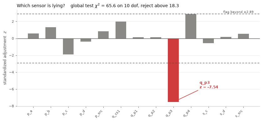
The global test compares the reconciliation objective against \(\chi^2\) on the degrees of redundancy: it says something is wrong. The measurement test standardizes each adjustment by its own standard deviation, \(z_i = (\hat x_i - y_i)/\sqrt{\Sigma_{adj,ii}}\), and points at the culprit — here q_p3 stands well clear of everything else.

Note that the second-largest \(|z|\) belongs to an innocent sensor. That is smearing: the adjustment had to go somewhere. Serial elimination discards the prime suspect and re-tests.

for step in serial_elimination(
    residual_fn, y_bad, sigma,
    names=layout.names, unmeasured_scale=layout.default_scale,
):
    removed = step.removed or "(none)"
    verdict = "REJECT" if step.detected else "accept"
    print(f"removed {removed:<8} chi2 = {step.statistic:7.3f} on {step.dof:2d} dof "
          f"-> {verdict}   next suspect: {step.suspect}")

removed (none)   chi2 =  65.583 on 10 dof -> REJECT   next suspect: q_p3
removed q_p3     chi2 =   8.729 on  9 dof -> accept   next suspect: None

Discarding q_p3 drops the statistic from rejection to a routine value, at the cost of one degree of redundancy. The data are clean — and the flow through p3 is still estimated, now from the balances alone rather than from a meter that was lying.

7. Estimating an unmeasured fouling factor

Pipes foul. Their effective resistance drifts above the design value, and nobody measures it directly. In this framework an unknown parameter is simply a variable with no measurement: give it \(\sigma = \infty\) and it is estimated rather than reconciled, in the same solve, with a standard error from the same covariance matrix.

Add an efficiency multiplier \(\eta\) on p3, where \(\eta > 1\) means more resistance.

# a network whose p3 really is 15% more resistive than the model believes
fouled = dg.GasNetwork(
    arcs=net.arcs,
    beta={**net.beta, "p3": net.beta["p3"] * 1.15},
    supply_kg_s=net.supply_kg_s,
)
fs_f, dec_f = dg.build_network_flowsheet(
    fouled, root="src", p_slack_pa=P_SLACK_PA, ratios=RATIOS
)
st_f = fs_f.solve(tol=1e-12, max_iter=500)

layout_eta = dg.gas_state_layout(net, efficiency_arcs=["p3"])
sigma_eta = dg.measurement_sigma(layout_eta)        # eta defaults to unmeasured

x_fouled = layout_eta.pack(
    verify.node_pressures_bar(st_f, dec_f),
    verify.arc_flows_kg_s(st_f, dec_f),
    fouled.supply_kg_s,
    {"eta_p3": 1.0},
)
y_fouled = dg.perturb(x_fouled, sigma_eta, jax.random.PRNGKey(3))

# the residual model still uses the CLEAN beta, so eta must absorb the fouling
res_eta = dg.reconcile_network(net, y_fouled, sigma_eta, layout_eta, ratios=RATIOS)

eta, sd = res_eta.x_named["eta_p3"], res_eta.std["eta_p3"]
print(f"estimated eta_p3 = {eta:.4f} +- {sd:.4f}   (true value 1.15)")
print(f"that is {abs(eta - 1.15) / sd:.2f} standard errors from the truth")
print(f"\ndegrees of redundancy: {res_eta.structure.degree_of_redundancy} "
      f"(estimating a parameter costs one)")

estimated eta_p3 = 1.1337 +- 0.0487   (true value 1.15)
that is 0.34 standard errors from the truth

degrees of redundancy: 9 (estimating a parameter costs one)

The fouling is recovered from pressures and flows that never mention it, with an honest uncertainty attached. Nothing about this was a separate “parameter estimation” step — it is the same least-squares problem with one fewer weight.

The complementary question is what happens to the reconciled state if a fixed parameter changes. That is a derivative, not an estimate, and params supplies it:

def q_p3_hat(efficiency):
    """Reconciled flow through p3 as a function of its fouling factor."""
    x, _ = solve_reconciliation(
        residual_fn, y, sigma, x0=x_true,
        scaling=res.scaling, params={"p3": efficiency}, n_steps=12,
    )
    return x[layout.index("q_p3")]

print(f"q_p3 at eta = 1.0      : {float(q_p3_hat(1.0)):.4f} kg/s")
print(f"d q_p3 / d eta         : {float(jax.grad(q_p3_hat)(1.0)):.4f} kg/s per unit eta")

q_p3 at eta = 1.0      : 55.6231 kg/s

d q_p3 / d eta         : -14.3876 kg/s per unit eta

Negative, as it must be: a dirtier pipe carries less of the loop’s flow. The gradient runs through the entire reconciliation — the Gauss-Newton iteration, the KKT solves, the constraint Jacobian — by the implicit function theorem.

8. Where estimation stops working

You cannot estimate everything. The KKT system is nonsingular if and only if the constraint Jacobian \(A\) has full row rank and its unmeasured columns have full column rank — the second is exactly the classical observability condition of data reconciliation. Solvability and observability are one test, and it runs before the solve, so an ill-posed problem is diagnosed rather than returning NaN.

Un-meter the whole loop — three flows and three pressures — while still asking for \(\eta\):

LOOP = ["q_p2", "q_p3", "q_p4", "p_b", "p_c", "p_d"]

sigma_blind = dg.measurement_sigma(layout_eta, unmeasured=LOOP)
try:
    dg.reconcile_network(net, y_fouled, sigma_blind, layout_eta, ratios=RATIOS)
except ReconciliationStructureError as err:
    print(err)

reconciliation problem is not solvable: 1 unmeasured variable(s) cannot be determined from the constraints. Unobservable: eta_p3. (10 equations, 7 measured and 7 unmeasured variables; rank(A)=10, rank(A_unmeasured)=6). Measure one of the variables above, give it a finite sigma as a prior, or remove it from the state.

Now drop \(\eta\) and un-meter the same six loop variables:

sigma_loop = dg.measurement_sigma(layout, unmeasured=LOOP)
res_loop = dg.reconcile_network(net, y, sigma_loop, layout, ratios=RATIOS)

print(f"solvable: {res_loop.structure.solvable}, "
      f"degrees of redundancy: {res_loop.structure.degree_of_redundancy}")
for name in LOOP:
    print(f"  {name:<6} = {res_loop.x_named[name]:8.3f}  +- {res_loop.std[name]:.3f}")

solvable: True, degrees of redundancy: 4
  q_p2   =   64.532  +- 0.383
  q_p3   =   55.935  +- 0.329
  q_p4   =   16.259  +- 0.871
  p_b    =   61.884  +- 0.277
  p_c    =   57.349  +- 0.312
  p_d    =   56.747  +- 0.317

Six unknowns are recoverable; seven are not. And the reason the six work is the compressor: \(p_b = 1.2\,p_a\) ties the loop’s pressures to the measured pressure upstream of the station. Remove that equation — as verify does, quite reasonably, for a sequential solve — and the loop’s pressure level floats free. The flow split is still fixed by the balances and the pipe laws; only the absolute pressures are lost.

The classification is available directly, for any variable:

print(res_loop.structure.summary())

degrees of redundancy : 4
equations             : 10
measured / unmeasured : 7 / 6
solvable              : True

variable             class                        redundancy
------------------------------------------------------------
p_a                  measured-redundant                0.408
p_b                  unmeasured-observable                  
p_c                  unmeasured-observable                  
p_d                  unmeasured-observable                  
p_src                measured-redundant                0.553
q_cs1                measured-redundant                0.640
q_p1                 measured-redundant                0.640
q_p2                 unmeasured-observable                  
q_p3                 unmeasured-observable                  
q_p4                 unmeasured-observable                  
s_c                  measured-redundant                0.460
s_d                  measured-redundant                0.460
s_src                measured-redundant                0.840

Estimating anyway, with a prior

Failing is not the only option. A finite \(\sigma\) on an unmetered variable is a Bayesian prior, and costs nothing extra — it is simply another measured entry. Instead of raising, a weakly identified parameter shrinks toward its prior.

Be careful what you conclude from it, though.

sigma_prior = dg.measurement_sigma(
    layout_eta, unmeasured=LOOP, sigma_eta=0.1     # a 10% prior on the fouling
)
res_prior = dg.reconcile_network(
    net, y_fouled, sigma_prior, layout_eta, ratios=RATIOS
)
print(f"eta_p3 = {res_prior.x_named['eta_p3']:.4f} +- {res_prior.std['eta_p3']:.4f}")
print(f"prior was          1.0000 +- 0.1000")
print(f"truth is           1.1500")
print(f"\ninformation gained from the data: "
      f"{100 * (1 - (res_prior.std['eta_p3'] / 0.1) ** 2):.1f}% of the prior variance")

eta_p3 = 1.0000 +- 0.1000
prior was          1.0000 +- 0.1000
truth is           1.1500

information gained from the data: 0.0% of the prior variance

The posterior is the prior, exactly — and it is wrong, because the truth is 1.15.

With the loop unmetered the data say nothing whatever about \(\eta\), so reconciliation returns what you told it to believe. This is the honest failure mode of a prior: it converts an error you would have noticed into an answer you might not question. The standard error is the tell — no reduction means no information — and the fix is not a better prior but a meter.

9. Which sensor should you buy?

The value of a meter is not its own accuracy but how much it sharpens the quantity you care about — a question the covariance answers before any money is spent. Rank candidate sensors by their effect on the fouling estimate, starting from the blind loop with the 10% prior on \(\eta\) from the previous cell. The percentages are therefore relative to that prior: a wider prior pushes every flow meter toward 100%, but the ranking holds.

ranked = sensor_ranking(
    dg.network_residual_fn(net, layout_eta, ratios=RATIOS),
    x_fouled, sigma_prior,
    target="eta_p3", candidates=LOOP, candidate_sigma=1.0,
    names=layout_eta.names,
)

print(f"{'add a meter on':<16} {'sd(eta)':>10} {'variance reduction':>20}")
print("-" * 50)
for d in ranked:
    print(f"{d['candidate']:<16} {d['sd_before']:.4f} -> {d['sd_after']:.4f}"
          f" {100 * d['variance_reduction']:14.1f} %")

add a meter on      sd(eta)   variance reduction
--------------------------------------------------
q_p3             0.1000 -> 0.0661           56.3 %
q_p2             0.1000 -> 0.0666           55.7 %
q_p4             0.1000 -> 0.0741           45.1 %
p_d              0.1000 -> 0.0968            6.4 %
p_c              0.1000 -> 0.0985            2.9 %
p_b              0.1000 -> 0.1000            0.0 %

fig, ax = plt.subplots(figsize=(8, 3.4))
cand = [d["candidate"] for d in ranked][::-1]
red = [100 * d["variance_reduction"] for d in ranked][::-1]
ax.barh(np.arange(len(cand)), red, height=0.6,
        color=[BLUE if v > 1 else GREY for v in red], edgecolor="none")
ax.set_yticks(np.arange(len(cand)))
ax.set_yticklabels(cand, fontsize=8.5)
ax.set_xlabel("reduction in the variance of $\\eta$  (%)", fontsize=9, color=INK_SOFT)
ax.set_title("Which meter would sharpen the fouling estimate most?",
             fontsize=10, color=INK, loc="left")
for i, v in enumerate(red):
    ax.text(v + 1, i, f"{v:.0f}%", va="center", fontsize=8, color=INK_SOFT)
ax.set_xlim(0, max(red) * 1.18)
tidy(ax, axis="x")
ax.tick_params(axis="y", length=0)
plt.tight_layout()
plt.show()

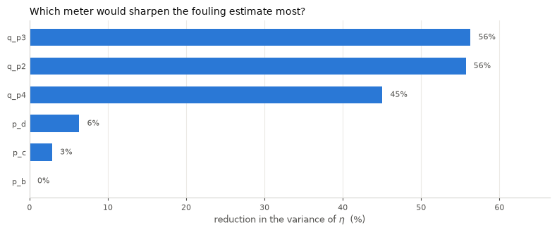
The loop flow meters are worth far more than the pressure transmitters, and p_b is worth nothing at all — it is already pinned by the compressor relation, so measuring it adds no information. That is the kind of conclusion that is expensive to reach empirically and nearly free to compute.

Summary

Question	Answer	Where it comes from
Do the measurements fit the model?	Global \(\chi^2\) test on the objective	global_test
What are the true values?	Constrained WLS via the KKT system	reconcile_network (reconcile underneath)
How good are the estimates?	\(\Sigma_{\hat x} = [K^{-1}]_{11}\)	res.covariance, res.std
Which sensor is lying?	Standardized adjustments	measurement_test, serial_elimination
What is the unknown parameter?	Give it \(\sigma = \infty\)	same solve
Can it be known at all?	\(\operatorname{rank}(A_U)\), before solving	res.structure, or a ReconciliationStructureError
Which meter should we add?	Covariance with and without	sensor_ranking
Is the model the thing that drifted?	The same tests, read over many days	monitor_network, reconcile_network_multi

What the differentiability bought

1. The constraint Jacobian is jax.jacobian(F) — no hand-derived analytical model per unit.

2. Gradients run through the reconciliation, so d(estimate)/d(parameter) is one jax.grad call.

3. Covariance can be obtained two independent ways, and their disagreement measures the model’s nonlinearity rather than a bug.

4. Joint parameter estimation is not a separate algorithm — it is one weight set to zero.

Practical notes

• Solve in bar and bar², not Pa. The KKT matrix mixes \(W\) (1/variable²) with \(A\) (residual/variable), so its conditioning depends on the unit system. Automatic scaling (on by default) removes most of that dependence; bar and bar² keep the raw numbers readable.

• Boundary flows belong in the state, not in the GasNetwork. Real nominations do not sum to zero, which is the whole point.

• Redundancy is uneven. A gross error on a weakly redundant sensor is caught with much less margin: the same 8σ bias gives \(z \approx -4.3\) on q_p4 (redundancy 0.58) against \(\approx -7.5\) on q_p3. Check the ranked \(z\) scores, not just the top one.

Next

Everything above is one snapshot, and it takes the model as correct. 29_model_updating.ipynb runs the same tests over a 45-day campaign, where the question inverts: the global test rejects, but is a sensor lying or has the model drifted? A single day cannot tell — monitor_network and diagnose() read the answer off the series — and once you are entitled to re-estimate a parameter, reconcile_network_multi pools the window into one solve instead of averaging daily estimates.