
Inverse Hessian-Vector Products and Newton Optimization#
This tutorial covers advanced automatic differentiation techniques:
Hessian-Vector Products (HVP): Compute H·v without forming H
Conjugate Gradient (CG): Solve linear systems iteratively
Inverse HVP: Compute H⁻¹·v using CG with HVPs
Newton Optimization: Second-order optimization using inverse HVP
Why This Matters#
Newton’s method for optimization computes: $\(x_{k+1} = x_k - H^{-1} \nabla f\)$
But forming and inverting H is O(n³). Using inverse HVP, we can compute the Newton step in O(n) per iteration!
import jax
import jax.numpy as jnp
from jax import grad, jvp, hessian
from jax.scipy.sparse.linalg import cg
import matplotlib.pyplot as plt

jax.config.update("jax_enable_x64", True)

print(f"JAX version: {jax.__version__}")
JAX version: 0.8.2
1. Review: Hessian-Vector Product (HVP)#
The HVP computes H·v without forming the full Hessian:
This uses forward-over-reverse mode: jvp of grad.
def hvp(f, x, v):
    """Hessian-vector product: H·v

    Computes H·v without forming H explicitly.
    Cost: O(n) - same as one gradient evaluation.
    """
    return jvp(grad(f), (x,), (v,))[1]


# Test function: Rosenbrock (classic optimization benchmark)
def rosenbrock(x):
    """f(x,y) = (1-x)² + 100(y-x²)²

    Minimum at (1, 1) with f(1,1) = 0.
    Has a curved valley that's hard to optimize.
    """
    return (1 - x[0])**2 + 100*(x[1] - x[0]**2)**2


x = jnp.array([0.0, 0.0])
v = jnp.array([1.0, 0.0])

# Compute HVP
hv = hvp(rosenbrock, x, v)
print(f"x = {x}")
print(f"v = {v}")
print(f"H·v = {hv}")

# Verify against full Hessian
H = hessian(rosenbrock)(x)
print(f"\nFull Hessian:\n{H}")
print(f"H @ v = {H @ v}  (should match H·v)")
WARNING:2026-01-10 20:24:08,117:jax._src.xla_bridge:852: An NVIDIA GPU may be present on this machine, but a CUDA-enabled jaxlib is not installed. Falling back to cpu.
x = [0. 0.]
v = [1. 0.]
H·v = [2. 0.]
Full Hessian:
[[  2.   0.]
 [  0. 200.]]
H @ v = [2. 0.]  (should match H·v)
2. Conjugate Gradient (CG) Algorithm#
CG solves the linear system \(A \cdot x = b\) iteratively, using only matrix-vector products.
Algorithm#
Initialize: x₀ = 0, r₀ = b, p₀ = r₀

For k = 0, 1, 2, ...
    αₖ = (rₖᵀrₖ) / (pₖᵀ A pₖ)     # step size
    xₖ₊₁ = xₖ + αₖ pₖ              # update solution
    rₖ₊₁ = rₖ - αₖ A pₖ            # update residual
    βₖ = (rₖ₊₁ᵀrₖ₊₁) / (rₖᵀrₖ)    # conjugacy parameter
    pₖ₊₁ = rₖ₊₁ + βₖ pₖ            # update search direction
Key property: Only needs one A·v product per iteration!
def cg_solve(A_matvec, b, x0=None, maxiter=100, tol=1e-10):
    """Conjugate Gradient solver.

    Solves A·x = b where A is symmetric positive definite.

    Args:
        A_matvec: Function computing A·v
        b: Right-hand side vector
        x0: Initial guess (default: zeros)
        maxiter: Maximum iterations
        tol: Convergence tolerance

    Returns:
        x: Solution
        info: Dictionary with convergence info
    """
    n = len(b)
    x = jnp.zeros(n) if x0 is None else x0
    r = b - A_matvec(x)  # residual
    p = r.copy()          # search direction
    rs_old = jnp.dot(r, r)

    residuals = [float(jnp.sqrt(rs_old))]

    for i in range(maxiter):
        Ap = A_matvec(p)
        alpha = rs_old / jnp.dot(p, Ap)
        x = x + alpha * p
        r = r - alpha * Ap
        rs_new = jnp.dot(r, r)

        residuals.append(float(jnp.sqrt(rs_new)))

        if jnp.sqrt(rs_new) < tol:
            break

        beta = rs_new / rs_old
        p = r + beta * p
        rs_old = rs_new

    return x, {'iterations': i+1, 'residuals': residuals}


# Example: Solve a simple linear system
A = jnp.array([[4., 1.], [1., 3.]])
b = jnp.array([1., 2.])

# Solve using our CG implementation
x_cg, info = cg_solve(lambda v: A @ v, b)

print(f"System: A·x = b")
print(f"A = \n{A}")
print(f"b = {b}")
print(f"\nCG solution: x = {x_cg}")
print(f"Iterations: {info['iterations']}")
print(f"\nVerification: A·x = {A @ x_cg}")
print(f"Direct solve: x = {jnp.linalg.solve(A, b)}")
System: A·x = b
A =
[[4. 1.]
 [1. 3.]]
b = [1. 2.]

CG solution: x = [0.09090909 0.63636364]
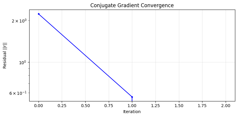
Iterations: 2

Verification: A·x = [1. 2.]
Direct solve: x = [0.09090909 0.63636364]
# Visualize CG convergence
plt.figure(figsize=(8, 4))
plt.semilogy(info['residuals'], 'b.-')
plt.xlabel('Iteration')
plt.ylabel('Residual ||r||')
plt.title('Conjugate Gradient Convergence')
plt.grid(True, alpha=0.3)
plt.tight_layout()
plt.show()
3. Inverse Hessian-Vector Product (IHVP)#
The inverse HVP computes \(H^{-1} \cdot v\) by solving:
Using CG with HVPs, we never form or invert H!
def ihvp(f, x, v, maxiter=50, tol=1e-8):
    """Inverse Hessian-vector product: H⁻¹·v

    Computes H⁻¹·v without forming or inverting H.
    Uses CG with HVPs internally.

    Args:
        f: Scalar function
        x: Point at which to evaluate Hessian
        v: Vector to multiply by H⁻¹
        maxiter: Maximum CG iterations
        tol: Convergence tolerance

    Returns:
        H⁻¹·v
    """
    # Define the Hessian-vector product operator
    def hvp_op(u):
        return hvp(f, x, u)

    # Solve H·result = v using CG
    result, _ = cg(hvp_op, v, maxiter=maxiter, tol=tol)
    return result


# Test inverse HVP
x = jnp.array([0.5, 0.5])
v = jnp.array([1.0, 2.0])

# Compute H⁻¹·v using our function
ihv = ihvp(rosenbrock, x, v)
print(f"x = {x}")
print(f"v = {v}")
print(f"H⁻¹·v = {ihv}")

# Verify against explicit inverse
H = hessian(rosenbrock)(x)
H_inv = jnp.linalg.inv(H)
print(f"\nFull Hessian:\n{H}")
print(f"\nExplicit H⁻¹·v = {H_inv @ v}  (should match)")

# Double-check: H·(H⁻¹·v) should equal v
print(f"\nVerification: H·(H⁻¹·v) = {hvp(rosenbrock, x, ihv)}")
print(f"Original v = {v}")
x = [0.5 0.5]
v = [1. 2.]
H⁻¹·v = [-0.03061224 -0.02061224]

Full Hessian:
[[ 102. -200.]
 [-200.  200.]]

Explicit H⁻¹·v = [-0.03061224 -0.02061224]  (should match)

Verification: H·(H⁻¹·v) = [1. 2.]
Original v = [1. 2.]
4. Newton Optimization#
Newton’s method uses the update:
where the Newton step \(\delta = -H^{-1} \nabla f\) is computed via inverse HVP.
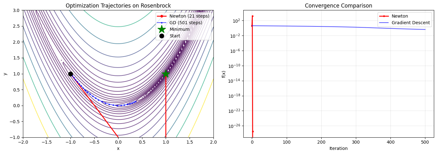
Comparison:#
Gradient descent: Uses only first-order info, slow near minimum
Newton’s method: Uses curvature (second-order), fast convergence
def newton_step(f, x):
    """Compute Newton step: δ = -H⁻¹·∇f"""
    g = grad(f)(x)
    return -ihvp(f, x, g)


def gradient_descent_step(f, x, lr=0.001):
    """Compute gradient descent step: δ = -lr·∇f"""
    g = grad(f)(x)
    return -lr * g


def optimize(f, x0, step_fn, n_steps=50):
    """Run optimization and track trajectory."""
    trajectory = [x0]
    x = x0
    for _ in range(n_steps):
        delta = step_fn(f, x)
        x = x + delta
        trajectory.append(x)
    return jnp.array(trajectory)


# Starting point
x0 = jnp.array([-1.0, 1.0])

# Run both optimizers
traj_newton = optimize(rosenbrock, x0, newton_step, n_steps=20)
traj_gd = optimize(rosenbrock, x0,
                   lambda f, x: gradient_descent_step(f, x, lr=0.002),
                   n_steps=500)

print(f"Starting point: {x0}")
print(f"True minimum: [1, 1]")
print(f"\nNewton (20 steps): {traj_newton[-1]}")
print(f"GD (500 steps):    {traj_gd[-1]}")
Starting point: [-1.  1.]
True minimum: [1, 1]
Newton (20 steps): [1. 1.]
GD (500 steps):    [0.36390293 0.1293884 ]
# Visualize optimization trajectories
fig, axes = plt.subplots(1, 2, figsize=(14, 5))

# Create contour plot
x_range = jnp.linspace(-2, 2, 100)
y_range = jnp.linspace(-1, 3, 100)
X, Y = jnp.meshgrid(x_range, y_range)
Z = jnp.array([[rosenbrock(jnp.array([xi, yi]))
                for xi, yi in zip(x_row, y_row)]
               for x_row, y_row in zip(X, Y)])

# Plot 1: Trajectories on contour
ax1 = axes[0]
ax1.contour(X, Y, Z, levels=jnp.logspace(-1, 3, 20), cmap='viridis', alpha=0.7)
ax1.plot(traj_newton[:, 0], traj_newton[:, 1], 'r.-',
         label=f'Newton ({len(traj_newton)} steps)', markersize=10, linewidth=2)
ax1.plot(traj_gd[::20, 0], traj_gd[::20, 1], 'b.-',
         label=f'GD ({len(traj_gd)} steps)', markersize=5, alpha=0.7)
ax1.plot(1, 1, 'g*', markersize=20, label='Minimum')
ax1.plot(x0[0], x0[1], 'ko', markersize=10, label='Start')
ax1.set_xlabel('x')
ax1.set_ylabel('y')
ax1.set_title('Optimization Trajectories on Rosenbrock')
ax1.legend()
ax1.set_xlim(-2, 2)
ax1.set_ylim(-1, 3)

# Plot 2: Convergence
ax2 = axes[1]
f_newton = [float(rosenbrock(x)) for x in traj_newton]
f_gd = [float(rosenbrock(x)) for x in traj_gd]
ax2.semilogy(f_newton, 'r.-', label='Newton', linewidth=2)
ax2.semilogy(f_gd, 'b-', label='Gradient Descent', alpha=0.7)
ax2.set_xlabel('Iteration')
ax2.set_ylabel('f(x)')
ax2.set_title('Convergence Comparison')
ax2.legend()
ax2.grid(True, alpha=0.3)

plt.tight_layout()
plt.show()
<cell_type>markdown</cell_type>## 5. Scaling: IHVP vs Naive Hessian Inverse
For large problems, explicit Hessian operations become prohibitive:
Operation |
Time Complexity |
Memory |
|---|---|---|
Form H |
O(n²) |
O(n²) |
Invert H (or solve) |
O(n³) |
O(n²) |
Single HVP |
O(n) |
O(n) |
IHVP via CG (k iters) |
O(kn) |
O(n) |
Key insight: The explicit method requires storing the full n×n Hessian matrix, while IHVP only needs a few vectors.
For n = 10,000 parameters:
Hessian storage: 800 MB (10,000² × 8 bytes)
IHVP storage: ~0.8 MB (just vectors)
When does IHVP win?
Small n (< 500): Explicit method is faster due to optimized BLAS
Large n (> 1000): IHVP wins on both time (O(kn) vs O(n³)) and memory (O(n) vs O(n²))
Memory-constrained: IHVP is essential when Hessian doesn’t fit in memory
import time
import tracemalloc

def benchmark_with_memory(n, n_trials=3):
    """Benchmark IHVP vs explicit inverse for dimension n.

    Returns timing and peak memory usage for both methods.
    """
    # Create a quadratic function with random Hessian
    key = jax.random.PRNGKey(42)
    A = jax.random.normal(key, (n, n))
    A = A @ A.T + jnp.eye(n)  # Make positive definite

    def quadratic(x):
        return 0.5 * x @ A @ x

    x = jnp.ones(n)
    v = jnp.ones(n)

    # Warm up JIT
    _ = ihvp(quadratic, x, v)
    _ = ihvp(quadratic, x, v)

    # Benchmark IHVP
    tracemalloc.start()
    start = time.time()
    for _ in range(n_trials):
        result_ihvp = ihvp(quadratic, x, v)
        result_ihvp.block_until_ready()  # Ensure computation completes
    time_ihvp = (time.time() - start) / n_trials
    _, peak_ihvp = tracemalloc.get_traced_memory()
    tracemalloc.stop()

    # Benchmark explicit method (form H, then solve)
    if n <= 3000:  # Skip for very large n
        # Warm up
        H = hessian(quadratic)(x)
        _ = jnp.linalg.solve(H, v)

        tracemalloc.start()
        start = time.time()
        for _ in range(n_trials):
            H = hessian(quadratic)(x)
            result_explicit = jnp.linalg.solve(H, v)
            result_explicit.block_until_ready()
        time_explicit = (time.time() - start) / n_trials
        _, peak_explicit = tracemalloc.get_traced_memory()
        tracemalloc.stop()
    else:
        time_explicit = None
        peak_explicit = None

    # Theoretical memory for Hessian: n² floats × 8 bytes
    hessian_memory = n * n * 8

    return {
        'n': n,
        'time_ihvp': time_ihvp,
        'time_explicit': time_explicit,
        'mem_ihvp': peak_ihvp,
        'mem_explicit': peak_explicit,
        'mem_hessian_theory': hessian_memory,
    }


# Run benchmarks for increasing problem sizes
print("Running benchmarks (this may take a minute)...")
print()

sizes = [100, 500, 1000, 1500, 2000, 2500, 3000]
results = []

for n in sizes:
    print(f"  n = {n}...", end=" ", flush=True)
    res = benchmark_with_memory(n)
    results.append(res)
    print("done")

print()
print("=" * 80)
print(f"{'n':>6} | {'IHVP (ms)':>10} | {'Explicit (ms)':>13} | {'Speedup':>8} | {'H memory':>10}")
print("=" * 80)

for r in results:
    t_i = r['time_ihvp'] * 1000
    t_e = r['time_explicit'] * 1000 if r['time_explicit'] else float('nan')
    speedup = r['time_explicit'] / r['time_ihvp'] if r['time_explicit'] else float('nan')
    mem_h = r['mem_hessian_theory'] / 1e6  # MB

    if r['time_explicit']:
        marker = " <-- IHVP wins!" if speedup > 1 else ""
        print(f"{r['n']:>6} | {t_i:>10.1f} | {t_e:>13.1f} | {speedup:>7.2f}x | {mem_h:>8.1f} MB{marker}")
    else:
        print(f"{r['n']:>6} | {t_i:>10.1f} | {'N/A':>13} | {'N/A':>8} | {mem_h:>8.1f} MB")

print("=" * 80)
print("\nNote: IHVP has constant overhead from CG iterations, but scales as O(kn)")
print("      Explicit scales as O(n²) for Hessian formation + O(n³) for solve")
Running benchmarks (this may take a minute)...

  n = 100...
done
  n = 500...
done
  n = 1000...
done
  n = 1500...
done
  n = 2000...
done
  n = 2500...
done
  n = 3000...
done

================================================================================
     n |  IHVP (ms) | Explicit (ms) |  Speedup |   H memory
================================================================================
   100 |      207.2 |          36.5 |    0.18x |      0.1 MB
   500 |      218.1 |          67.2 |    0.31x |      2.0 MB
  1000 |      222.3 |         190.3 |    0.86x |      8.0 MB
  1500 |      236.6 |         189.8 |    0.80x |     18.0 MB
  2000 |      252.7 |         265.9 |    1.05x |     32.0 MB <-- IHVP wins!
  2500 |      333.1 |         388.0 |    1.16x |     50.0 MB <-- IHVP wins!
  3000 |      365.1 |         687.6 |    1.88x |     72.0 MB <-- IHVP wins!
================================================================================

Note: IHVP has constant overhead from CG iterations, but scales as O(kn)
      Explicit scales as O(n²) for Hessian formation + O(n³) for solve
# Visualize timing and memory comparison
fig, axes = plt.subplots(1, 2, figsize=(14, 5))

ns = [r['n'] for r in results]
times_ihvp = [r['time_ihvp'] * 1000 for r in results]
times_explicit = [r['time_explicit'] * 1000 if r['time_explicit'] else None for r in results]
mem_hessian = [r['mem_hessian_theory'] / 1e6 for r in results]  # MB

# Plot 1: Timing comparison
ax1 = axes[0]
ax1.loglog(ns, times_ihvp, 'b.-', markersize=10, linewidth=2, label='IHVP (CG)')
valid_explicit = [(n, t) for n, t in zip(ns, times_explicit) if t is not None]
if valid_explicit:
    ax1.loglog([x[0] for x in valid_explicit], [x[1] for x in valid_explicit],
               'r.-', markersize=10, linewidth=2, label='Explicit H⁻¹')

# Add reference lines for scaling
n_ref = jnp.array([100, 3000])
ax1.loglog(n_ref, 30 * (n_ref / 100)**1, 'g--', alpha=0.5, label='O(n)')
ax1.loglog(n_ref, 5 * (n_ref / 100)**2, 'm--', alpha=0.5, label='O(n²)')

ax1.set_xlabel('Problem size n', fontsize=12)
ax1.set_ylabel('Time (ms)', fontsize=12)
ax1.set_title('Timing: IHVP vs Explicit Hessian Inverse', fontsize=12)
ax1.legend()
ax1.grid(True, alpha=0.3)

# Mark crossover point
crossover_n = None
for i, r in enumerate(results):
    if r['time_explicit'] and r['time_explicit'] > r['time_ihvp']:
        crossover_n = r['n']
        break
if crossover_n:
    ax1.axvline(x=crossover_n, color='gray', linestyle=':', alpha=0.7)
    ax1.annotate(f'Crossover\nn≈{crossover_n}', xy=(crossover_n, 50), fontsize=10)

# Plot 2: Memory comparison
ax2 = axes[1]

# IHVP memory: O(n) - just vectors
mem_ihvp_theory = [8 * n * 10 / 1e6 for n in ns]  # ~10 vectors of size n

ax2.loglog(ns, mem_hessian, 'r.-', markersize=10, linewidth=2, label='Explicit: O(n²) for Hessian')
ax2.loglog(ns, mem_ihvp_theory, 'b.-', markersize=10, linewidth=2, label='IHVP: O(n) vectors only')

ax2.set_xlabel('Problem size n', fontsize=12)
ax2.set_ylabel('Memory (MB)', fontsize=12)
ax2.set_title('Memory Usage: IHVP vs Explicit Method', fontsize=12)
ax2.legend()
ax2.grid(True, alpha=0.3)

# Add annotations for largest size
max_idx = -1
ax2.annotate(f'n={ns[max_idx]}:\n{mem_hessian[max_idx]:.0f} MB',
             xy=(ns[max_idx], mem_hessian[max_idx]), xytext=(ns[max_idx]//2, mem_hessian[max_idx]*1.5),
             arrowprops=dict(arrowstyle='->', color='red'),
             fontsize=10, color='red')
ax2.annotate(f'n={ns[max_idx]}:\n{mem_ihvp_theory[max_idx]:.2f} MB',
             xy=(ns[max_idx], mem_ihvp_theory[max_idx]), xytext=(ns[max_idx]//2, mem_ihvp_theory[max_idx]/3),
             arrowprops=dict(arrowstyle='->', color='blue'),
             fontsize=10, color='blue')

plt.tight_layout()
plt.show()

# Print memory savings
print(f"\nMemory comparison at n={ns[-1]}:")
print(f"  Explicit method needs: {mem_hessian[-1]:.1f} MB (to store Hessian)")
print(f"  IHVP method needs:     {mem_ihvp_theory[-1]:.2f} MB (just vectors)")
print(f"  Memory savings:        {mem_hessian[-1] / mem_ihvp_theory[-1]:.0f}x less memory with IHVP")
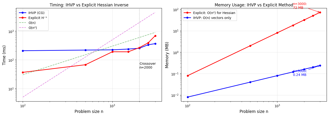
Memory comparison at n=3000:
  Explicit method needs: 72.0 MB (to store Hessian)
  IHVP method needs:     0.24 MB (just vectors)
  Memory savings:        300x less memory with IHVP
6. Application: Newton-CG for Large-Scale Optimization#
For real applications, we combine:
Line search: Ensure sufficient decrease
Trust region: Limit step size
Preconditioning: Accelerate CG convergence
def newton_cg_optimize(f, x0, maxiter=100, gtol=1e-6, verbose=True):
    """Newton-CG optimizer with backtracking line search.

    Args:
        f: Objective function
        x0: Initial point
        maxiter: Maximum iterations
        gtol: Gradient tolerance for convergence
        verbose: Print progress

    Returns:
        x: Optimized point
        info: Optimization info
    """
    x = x0
    history = {'f': [], 'gnorm': []}

    for i in range(maxiter):
        g = grad(f)(x)
        gnorm = jnp.linalg.norm(g)
        fval = f(x)

        history['f'].append(float(fval))
        history['gnorm'].append(float(gnorm))

        if verbose and i % 5 == 0:
            print(f"Iter {i:3d}: f = {fval:.6e}, ||g|| = {gnorm:.6e}")

        if gnorm < gtol:
            if verbose:
                print(f"Converged at iteration {i}")
            break

        # Newton direction via CG
        direction = -ihvp(f, x, g)

        # Backtracking line search
        alpha = 1.0
        c = 1e-4  # Armijo constant
        rho = 0.5  # Backtracking factor

        while f(x + alpha * direction) > fval + c * alpha * jnp.dot(g, direction):
            alpha *= rho
            if alpha < 1e-10:
                break

        x = x + alpha * direction

    return x, history


# Optimize Rosenbrock
x0 = jnp.array([-1.5, 1.5])
x_opt, history = newton_cg_optimize(rosenbrock, x0, maxiter=50, verbose=True)

print(f"\nOptimum: {x_opt}")
print(f"f(x*) = {rosenbrock(x_opt):.2e}")
Iter 0: f = 6.250000e+01, ||g|| = 4.790877e+02
Iter 5: f = 2.883150e+00, ||g|| = 6.902294e+00
Iter 10: f = 9.529114e-01, ||g|| = 1.228755e+01
Iter 15: f = 6.708411e-02, ||g|| = 7.014664e-01
Iter 20: f = 1.993389e-05, ||g|| = 1.210767e-01
Converged at iteration 23

Optimum: [1. 1.]
f(x*) = 9.48e-24
Summary#
Concept |
Formula |
JAX Implementation |
|---|---|---|
Gradient |
∇f |
|
Hessian-vector product |
H·v |
|
Inverse Hessian-vector product |
H⁻¹·v |
|
Newton step |
-H⁻¹·∇f |
|
Key takeaways:
CG solves linear systems using only matrix-vector products
IHVP computes H⁻¹·v in O(kn) vs O(n³) for explicit inversion
Newton-CG enables second-order optimization for large problems
All operations are differentiable in JAX!