
Flowsheet Optimization with pounce and asdex#
This notebook connects three libraries:
difflow builds the process model,
asdex detects the sparsity structure of the model’s derivatives, symbolically,
pounce solves the resulting nonlinear program.
JAX is the glue. Every difflow model is a traced JAX function, so the objective gradient, the constraint Jacobian and the Lagrangian Hessian that an interior-point solver needs are all available by automatic differentiation – exact, not finite-differenced, and not hand-coded.
The design problem#
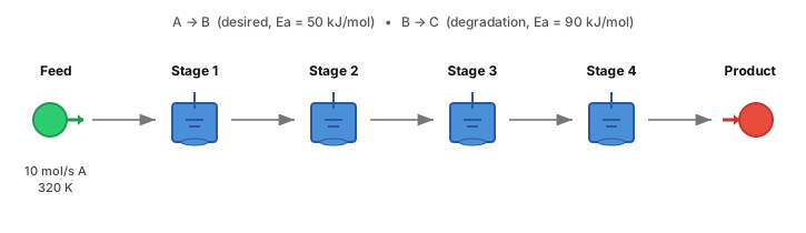
A train of four CSTRs runs a desired reaction alongside a thermal degradation reaction:
Raising the temperature shrinks the reactor volume needed to hit a conversion spec, but the degradation reaction has the higher activation energy, so it accelerates faster than the desired one and destroys product. Each stage gets its own volume and its own temperature, so the optimizer can shape a temperature profile down the train.
import jax
import jax.numpy as jnp
import numpy as np
import matplotlib.pyplot as plt

jax.config.update("jax_enable_x64", True)

from difflow.streams import make_stream
from difflow.thermo import IdealThermo, SpeciesData
from difflow.units.cstr import CSTR, CSTRParams

import asdex
from pounce.jax import from_jax
1. The difflow model#
Standard difflow setup: species data, an ideal thermo package, a stoichiometry matrix whose columns are the two reactions, and a JAX-traced rate law.
R = 8.314
SPECIES = ["A", "B", "C"]
N_SPECIES = len(SPECIES)
N_STAGES = 4

species_data = {
    s: SpeciesData(
        name=s, MW=100.0, Cp_coeffs=(75.0, 0.0, 0.0, 0.0),
        Hvap_coeffs=(30000.0, 0.38, 450.0), antoine_coeffs=(10.0, 2800.0, -40.0),
    )
    for s in SPECIES
}
thermo = IdealThermo(species_data)

# Columns are reactions, rows are species: A -> B, then B -> C.
STOICH = jnp.array([
    [-1.0,  0.0],   # A
    [ 1.0, -1.0],   # B
    [ 0.0,  1.0],   # C
])

RATE_PARAMS = {
    "A1": 1.0e6, "Ea1": 50_000.0,   # desired
    "A2": 5.0e9, "Ea2": 90_000.0,   # degradation -- higher Ea, so T-sensitive
}

FEED = 10.0        # mol/s of pure A
FEED_T = 320.0     # K
P0 = 101325.0      # Pa
QV = 0.01          # m^3/s -- sets stage residence time tau_k = V_k / QV


def rate_fn(C, T, p):
    """First-order rates for both reactions (mol/m^3/s)."""
    k1 = p["A1"] * jnp.exp(-p["Ea1"] / (R * T))
    k2 = p["A2"] * jnp.exp(-p["Ea2"] / (R * T))
    return jnp.array([k1 * C["A"], k2 * C["B"]])


def make_reactor(V):
    params = CSTRParams(
        V=V, rate_fn=rate_fn, stoich=STOICH, rate_params=RATE_PARAMS,
        species_order=SPECIES, dH_rxn=jnp.array([-50000.0, -20000.0]),
    )
    return CSTR(params, thermo=thermo, mode="isothermal")
The process#
Four CSTRs in series, drawn with difflow’s own unit-operation icons
(difflow.visualization.get_icon_svg). Each stage has its own volume and its
own temperature, so the optimizer has \(2N = 8\) degrees of freedom to shape the
train – plus the stream variables, once we move to the equation-oriented form
below.
from IPython.display import SVG, display
from difflow.visualization import get_icon_svg
ICON, GAP, Y = 60, 125, 78
def _icon(name, x, y):
"""Place one of difflow's 60x60 unit icons at (x, y)."""
s = get_icon_svg(name)
return f'<g transform="translate({x},{y})">{s[s.index(">") + 1:s.rindex("</svg>")]}</g>'
def draw_process(V=None, T=None):
"""Process flow diagram of the reactor train, optionally annotated."""
xs = [20 + GAP * i for i in range(N_STAGES + 2)]
W, H = xs[-1] + ICON + 20, 210
p = [f'<svg xmlns="http://www.w3.org/2000/svg" width="{W}" height="{H}" viewBox="0 0 {W} {H}">',
'<style>text{font-family:-apple-system,Segoe UI,Helvetica,sans-serif}'
'.l{font-size:11px;fill:#444;text-anchor:middle}'
'.v{font-size:11px;fill:#2c5aa0;text-anchor:middle}'
'.h{font-size:12px;fill:#111;text-anchor:middle;font-weight:600}'
'.r{font-size:12px;fill:#555;text-anchor:middle}</style>',
'<defs><marker id="ar" markerWidth="9" markerHeight="9" refX="8" refY="3" orient="auto">'
'<path d="M0,0 L8,3 L0,6 z" fill="#777"/></marker></defs>',
f'<text class="r" x="{W/2}" y="24">A → B  (desired, Ea = 50 kJ/mol)'
'   •   B → C  (degradation, Ea = 90 kJ/mol)</text>']
for i in range(N_STAGES + 1):
p.append(f'<line x1="{xs[i]+ICON+3}" y1="{Y+30}" x2="{xs[i+1]-5}" y2="{Y+30}" '
'stroke="#777" stroke-width="1.6" marker-end="url(#ar)"/>')
for i, (nm, x) in enumerate(zip(["Feed"] + ["CSTR"] * N_STAGES + ["Product"], xs)):
p.append(_icon(nm, x, Y))
c = x + ICON / 2
if 1 <= i <= N_STAGES:
k = i - 1
p.append(f'<text class="h" x="{c}" y="{Y-10}">Stage {k+1}</text>')
if V is not None:
p.append(f'<text class="v" x="{c}" y="{Y+ICON+20}">V = {V[k]:.3f} m³</text>')
p.append(f'<text class="v" x="{c}" y="{Y+ICON+35}">T = {T[k]:.1f} K</text>')
p.append(f'<text class="h" x="{xs[0]+ICON/2}" y="{Y-10}">Feed</text>')
p.append(f'<text class="l" x="{xs[0]+ICON/2}" y="{Y+ICON+20}">{FEED:.0f} mol/s A</text>')
p.append(f'<text class="l" x="{xs[0]+ICON/2}" y="{Y+ICON+35}">{FEED_T:.0f} K</text>')
p.append(f'<text class="h" x="{xs[-1]+ICON/2}" y="{Y-10}">Product</text>')
p.append('</svg>')
return "\n".join(p)
SVG(draw_process())
2. Why an equation-oriented formulation#
There are two ways to hand this model to an optimizer.
Sequential-modular. Call reactor(inlet, T_spec=...) and let difflow solve
the reactor internally. The decision variables are just \((V_k, T_k)\), and the
reactor’s material balance is closed by an inner Newton solve. This works fine
with pounce, but the inner solve is opaque to sparsity detection: it emits a
linear_solve primitive into the jaxpr (via optimistix/lineax) that stock asdex
has no handler for. That is a missing handler rather than a hard limit – see the
closing note, where an eight-line conservative rule recovers the structure exactly
– but out of the box it stops detection. There is also little for asdex to find:
with only \(2N\) variables the Jacobian is nearly dense.
Equation-oriented. Promote the stream variables to decision variables and add the model equations as equality constraints. The model is now a set of explicit residuals – no inner solver – so asdex can trace it, and the Jacobian is large and genuinely sparse because stage \(k\) only touches stages \(k-1\) and \(k\). This is how full-space process optimizers work, and it is the formulation where sparsity detection earns its keep.
difflow exposes exactly what we need: CSTR.eo_residuals returns the residual
form of the unit.
Per stage the unknowns are \([V_k,\ T_k,\ F_{A,k},\ F_{B,k},\ F_{C,k}]\), so \(n = 5N = 20\). The constraints are \(N\) blocks of 3 material balances plus the conversion spec, so \(m = 3N + 1 = 13\).
N_VARS = 5  # V, T, F_A, F_B, F_C per stage
n = N_STAGES * N_VARS
m = N_STAGES * N_SPECIES + 1


def stage(z, k):
    """Unpack stage k: returns (V, T, F) with F = [F_A, F_B, F_C]."""
    b = k * N_VARS
    return z[b], z[b + 1], z[b + 2:b + 5]


def residuals(z):
    """Material-balance residuals for the whole train, straight from difflow."""
    out = []
    prev = make_stream({"A": FEED, "B": 0.0, "C": 0.0}, T=FEED_T, P=P0)

    for k in range(N_STAGES):
        V, T, F = stage(z, k)
        outlet = make_stream({"A": F[0], "B": F[1], "C": F[2]}, T=T, P=P0)
        r = make_reactor(V).eo_residuals([prev], [outlet], volumetric_flow=QV)
        # eo_residuals returns n_species material balances plus a T row and a P
        # row. Here T is a decision variable and P is fixed, so those two rows
        # are identities (0 = 0) -- keep only the material balances.
        out.append(r[:N_SPECIES])
        prev = outlet

    return jnp.concatenate(out)


def conversion(z):
    """Overall conversion of A across the train."""
    return (FEED - stage(z, N_STAGES - 1)[2][0]) / FEED


def g(z):
    """Constraint vector: model residuals, then the conversion spec."""
    return jnp.concatenate([residuals(z), jnp.atleast_1d(conversion(z))])


print(f"n = {n} variables, m = {m} constraints")
n = 20 variables, m = 13 constraints
3. The objective#
Profit per second: revenue from B, less feedstock and annualized reactor capital. Capital scales as \(V^{0.6}\), the usual economy-of-scale exponent. Note that nothing penalizes temperature directly – the only reason not to run hot is that it destroys product.
PRICE_B = 2.0     # $/mol of B sold
PRICE_A = 0.60    # $/mol of A fed
CAPITAL = 1.5     # $/s per (m^3)^0.6, annualized


def profit(z):
    """Profit rate ($/s)."""
    F_B = stage(z, N_STAGES - 1)[2][1]
    capital = sum(CAPITAL * stage(z, k)[0] ** 0.6 for k in range(N_STAGES))
    return PRICE_B * F_B - PRICE_A * FEED - capital


def f(z):
    """pounce minimizes, so minimize the negative profit."""
    return -profit(z)


# Starting point: a rough guess, not feasible -- the solver closes the residuals.
z0 = jnp.array([0.5, 360.0, 5.0, 4.0, 0.5] * N_STAGES)

print(f"profit(z0)   = {float(profit(z0)):+.4f} $/s")
print(f"|residuals|  = {float(jnp.linalg.norm(residuals(z0))):.3f}  (infeasible start)")
profit(z0) = -1.9585 $/s
|residuals| = 36.424 (infeasible start)
4. Sparsity detection with asdex#
asdex.jacobian_sparsity analyzes the computation graph rather than
evaluating derivatives, so the pattern it returns is valid for all inputs, and
it never has to evaluate the model at a point where it might not be defined.
That last part matters more than it sounds. pounce’s own built-in fallback discovers sparsity by probing derivatives at random \(\mathcal{N}(0,1)\) points – which for a process model means \(T \approx -1.3\) K, where the Arrhenius terms overflow and the model blows up. Symbolic detection sidesteps that entirely.
For the Lagrangian Hessian, pounce needs the union of the structures of \(\nabla^2 f\) and each \(\nabla^2 g_i\). Taking \(\lambda = 1\) gives exactly that union.
jac_pattern = asdex.jacobian_sparsity(g, z0)


def lagrangian(z):
    """Structural stand-in for the Lagrangian: lambda = 1 gives the union."""
    return f(z) + jnp.sum(g(z))


hess_pattern = asdex.hessian_sparsity(lagrangian, z0)

print(f"Jacobian: {jac_pattern.m} x {jac_pattern.n}, "
      f"{jac_pattern.nnz} nonzeros ({jac_pattern.density:.1%} dense)")
print(f"Hessian:  {hess_pattern.m} x {hess_pattern.n}, "
      f"{hess_pattern.nnz} nonzeros ({hess_pattern.density:.1%} dense)")
Jacobian: 13 x 20, 62 nonzeros (23.8% dense)
Hessian:  20 x 20, 48 nonzeros (12.0% dense)
fig, axes = plt.subplots(1, 2, figsize=(11, 4.5))

axes[0].spy(np.asarray(jac_pattern.todense()), markersize=8)
axes[0].set_title(f"Constraint Jacobian ({jac_pattern.density:.1%} dense)")
axes[0].set_xlabel("variable")
axes[0].set_ylabel("constraint")

axes[1].spy(np.asarray(hess_pattern.todense()), markersize=8)
axes[1].set_title(f"Lagrangian Hessian ({hess_pattern.density:.1%} dense)")
axes[1].set_xlabel("variable")
axes[1].set_ylabel("variable")

for ax in axes:
    for b in range(1, N_STAGES):
        ax.axvline(b * N_VARS - 0.5, color="0.8", lw=0.8, zorder=0)

fig.suptitle("Structure detected by asdex -- the block-banded stage coupling")
fig.tight_layout()
plt.show()
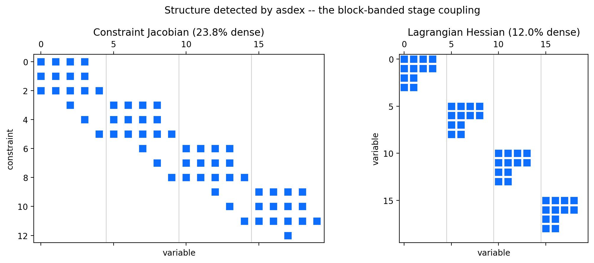
The block structure is the flowsheet topology made visible: each stage’s three material balances touch only that stage’s five variables plus the two inlet flows it inherits from the stage upstream. The last Jacobian row is the conversion spec, which touches a single variable (\(F_A\) in the final stage).
A sparsity pattern is only safe if it is a superset of the true structure – a missing entry silently drops a derivative. asdex claims its pattern holds for all inputs; let’s check that against a dense AD Jacobian.
(This notebook does the detection by hand to show what it is. In library
code, difflow.solvers.as_nlp derives both patterns this way by default and
validates them, and difflow.solvers.detect_patterns(f, g, x0, m) does the
same for a model you built yourself.)
J_pattern = np.asarray(jac_pattern.todense()) != 0
J_true = np.abs(np.asarray(jax.jacobian(g)(z0))) > 0

print(f"superset of the true structure: {bool((J_true <= J_pattern).all())}")
print(f"asdex {J_pattern.sum()} nonzeros | actually nonzero at z0 {J_true.sum()} "
      f"| dense would be {n * m}")
superset of the true structure: True
asdex 62 nonzeros | actually nonzero at z0 54 | dense would be 260
A valid superset, and a third of the dense cost. The eight extra entries are structurally-possible couplings that happen to evaluate to zero at this particular point – exactly the conservative side to err on.
5. Solve with pounce#
from_jax builds a pounce.Problem, deriving the gradient, Jacobian and
Lagrangian Hessian from f and g with jax.grad/jacrev/hessian.
Passing the patterns skips pounce’s own probe entirely, and sparse=True
switches the per-iteration derivatives to CPR-style colored AD – one
JVP/HVP per color instead of building the dense matrix and slicing it.
The equality constraints are the model residuals, so cl = cu = 0 for those
rows. The conversion spec gets [0.97, 1.0].
rows, cols = np.nonzero(J_pattern)
hrows, hcols = np.nonzero(np.asarray(hess_pattern.todense()) != 0)

# Bounds, per stage: V (m^3), T (K), then the three species flows (mol/s).
lb = jnp.array([0.01, 320.0, 0.0, 0.0, 0.0] * N_STAGES)
ub = jnp.array([5.00, 420.0, FEED, FEED, FEED] * N_STAGES)

# Residual rows are equalities; the last row is the conversion spec.
cl = jnp.concatenate([jnp.zeros(N_STAGES * N_SPECIES), jnp.array([0.97])])
cu = jnp.concatenate([jnp.zeros(N_STAGES * N_SPECIES), jnp.array([1.00])])

problem = from_jax(
    f, g, n=n, m=m, lb=lb, ub=ub, cl=cl, cu=cu,
    sparse=True,                       # colored AD using the patterns below
    jac_pattern=(rows, cols),          # from asdex -- no probing
    hess_pattern=(hrows, hcols),       # pounce folds this onto the lower triangle
)
problem.add_option("print_level", 0)
problem.add_option("tol", 1e-8)

z, info = problem.solve(x0=z0)
print(f"pounce: {info['status_msg']}")
pounce: Solve_Succeeded
print(f"profit       = {float(profit(z)):+.4f} $/s "
      f"(started at {float(profit(z0)):+.4f})")
print(f"conversion   = {float(conversion(z)):.4f}   (spec: >= 0.97)")
print(f"|residuals|  = {float(jnp.linalg.norm(residuals(z))):.2e}   (model is satisfied)")
print()
print(f"{'stage':>6} {'V (m^3)':>9} {'tau (s)':>9} {'T (K)':>8} "
      f"{'F_A':>7} {'F_B':>7} {'F_C':>7}")
for k in range(N_STAGES):
    V, T, F = stage(z, k)
    print(f"{k + 1:>6} {float(V):>9.4f} {float(V) / QV:>9.1f} {float(T):>8.1f} "
          f"{float(F[0]):>7.3f} {float(F[1]):>7.3f} {float(F[2]):>7.3f}")

F_B_final = float(stage(z, N_STAGES - 1)[2][1])
print(f"\nselectivity  = {F_B_final / (FEED * float(conversion(z))):.4f} "
      f"mol B per mol A converted")
profit       = +10.4739 $/s (started at -1.9585)
conversion   = 0.9700   (spec: >= 0.97)
|residuals|  = 2.07e-09   (model is satisfied)

 stage   V (m^3)   tau (s)    T (K)     F_A     F_B     F_C
     1    0.0703       7.0    386.0   4.536   5.340   0.124
     2    0.1159      11.6    377.8   1.876   7.836   0.288
     3    0.1357      13.6    375.3   0.754   8.781   0.465
     4    0.1439      14.4    374.3   0.300   9.056   0.644

selectivity  = 0.9336 mol B per mol A converted
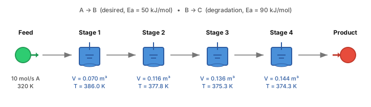
The same process diagram, now annotated with the optimal design:
V = [float(stage(z, k)[0]) for k in range(N_STAGES)]
T = [float(stage(z, k)[1]) for k in range(N_STAGES)]

SVG(draw_process(V, T))
F = np.array([[float(v) for v in stage(z, k)[2]] for k in range(N_STAGES)])
stages = np.arange(1, N_STAGES + 1)

fig, axes = plt.subplots(1, 3, figsize=(13, 4))

axes[0].bar(stages, V, color="steelblue")
axes[0].set(xlabel="stage", ylabel="volume (m$^3$)", title="Reactor volumes",
            xticks=stages)

axes[1].plot(stages, T, "o-", color="firebrick")
axes[1].set(xlabel="stage", ylabel="temperature (K)",
            title="Optimal temperature profile", xticks=stages)

for i, s in enumerate(SPECIES):
    axes[2].plot(np.r_[0, stages], np.r_[FEED if s == "A" else 0.0, F[:, i]],
                 "o-", label=s)
axes[2].set(xlabel="stage", ylabel="molar flow (mol/s)", title="Composition profile",
            xticks=np.r_[0, stages])
axes[2].legend()

fig.tight_layout()
plt.show()
What the optimizer found#
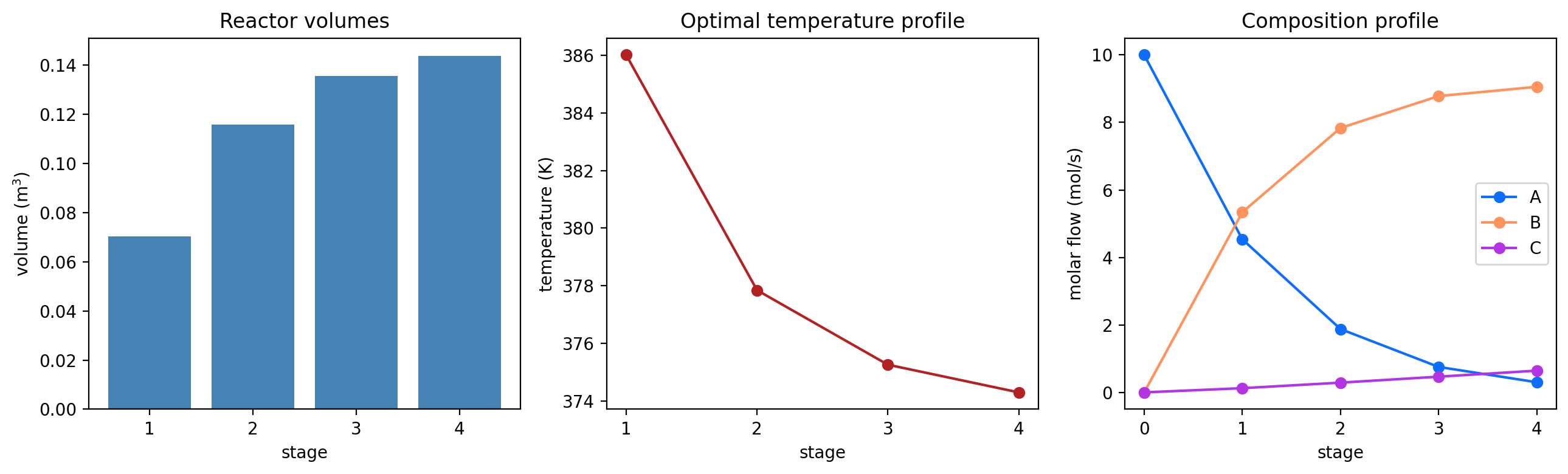
The temperature profile is decreasing down the train, and that is the whole story of this problem. Early on the stream is mostly A and there is little B to lose, so it pays to run hot and drive the desired reaction. As B accumulates, the degradation reaction – with its higher activation energy – becomes the dominant risk, so the optimal policy cools the later stages to protect the product. The volumes grow down the train to compensate for the slower kinetics.
Nobody encoded that policy. It falls out of maximizing profit subject to the model equations, with every derivative supplied by AD through the difflow model.
Summary of the three-library split#
Library |
Role |
Entry point |
|---|---|---|
difflow |
the process model, as explicit residuals |
|
asdex |
sparsity structure, from the computation graph |
|
pounce |
the NLP solve |
|
Three practical notes if you adapt this:
Stock asdex needs a solver-free model, but only because of one missing handler. difflow’s sequential-modular calls close their balances with
optimistix.Newton, which emits alinear_solveprimitive asdex does not handle. This is not a fundamental limitation. Adding a conservative rule – every output of the solve depends on every input – is correct, since \(A^{-1}\) of an irreducible sparse matrix is dense, and it recovers the exact block-triangular structure of a sequential-modular reactor train. One caveat if you try it: propagate dependence only to inexact (floating-point) outputs. lineax also returns integer status and stats, and marking those input-dependent poisons optimistix’s loop bookkeeping and trips asdex’sdynamic_slicecheck.Equation-oriented is still the better formulation here. The inner solve genuinely couples every variable in its block, so sequential-modular yields a denser pattern than the residual form – the inner solve hides structure that
eo_residualsexposes.A supplied pattern is a promise pounce does not check. It must be a superset of the true structure; extra entries cost a little, missing entries are silently wrong. The verification cell above is worth keeping.
Expect a superset, not the tightest pattern. asdex propagates dependence through the computation graph, so it reports what could couple. It cannot see algebraic cancellation: for first-order kinetics a stage’s fractional conversion is \(X = Vk/(\dot{V} + Vk)\), independent of its inlet flow, so upstream dependence cancels exactly – a fact no graph-reachability analysis can discover. That is the correct, safe direction to be wrong in.
Requirements#
pip install pounce-solver[jax] asdex
asdex >= 0.5.2 requires jax >= 0.11; on jax 0.10 install asdex == 0.5.1.