
Tutorial 25: Accessing Intermediate Derivatives#
In complex computations, you often need derivatives not just of the final output, but of intermediate values within the computation. This tutorial covers:
has_aux- Return intermediates alongside gradientsvalue_and_grad- Get both value and gradientJacobians of intermediate quantities
Gradient checkpointing with intermediate access
Custom VJP for intermediate gradients
Sensitivity of intermediates to parameters
Chemical engineering example: Reactor cascade analysis
import jax
import jax.numpy as jnp
from jax import grad, jacobian, vmap, jit, value_and_grad
from jax import custom_vjp
from functools import partial
import matplotlib.pyplot as plt

jax.config.update('jax_enable_x64', True)
1. The has_aux Pattern#
The most common way to get intermediate values during gradient computation is using has_aux=True. Your function returns (output, auxiliary_data), and JAX differentiates only through output.
# Basic has_aux example
def computation_with_intermediates(x):
    """A multi-step computation where we want intermediate values."""
    h1 = jnp.sin(x)           # First intermediate
    h2 = h1 ** 2              # Second intermediate
    h3 = jnp.exp(-h2)         # Third intermediate
    output = h3.sum()         # Final scalar output

    # Return output AND intermediates
    intermediates = {'h1': h1, 'h2': h2, 'h3': h3}
    return output, intermediates

# Create gradient function that returns auxiliaries
grad_fn = grad(lambda x: computation_with_intermediates(x)[0], has_aux=True)

# But wait - this doesn't work as expected!
# has_aux expects the function itself to return (value, aux)

# Correct approach:
def grad_with_aux(f):
    """Wrapper to get gradients with auxiliary outputs."""
    def f_for_grad(x):
        out, aux = f(x)
        return out, aux
    return grad(f_for_grad, has_aux=True)

# Test
x = jnp.array([0.5, 1.0, 1.5])
gradient, intermediates = grad(computation_with_intermediates, has_aux=True)(x)

print("Input x:", x)
print("\nIntermediate values:")
for name, value in intermediates.items():
    print(f"  {name}: {value}")
print(f"\nGradient d(output)/dx: {gradient}")
WARNING:2026-01-10 21:03:00,025:jax._src.xla_bridge:852: An NVIDIA GPU may be present on this machine, but a CUDA-enabled jaxlib is not installed. Falling back to cpu.
Input x: [0.5 1.  1.5]

Intermediate values:
  h1: [0.47942554 0.84147098 0.99749499]
  h2: [0.22984885 0.70807342 0.99499625]
  h3: [0.79465371 0.4925923  0.36972483]

Gradient d(output)/dx: [-0.66867804 -0.44791291 -0.05217557]
# Practical example: Neural network with intermediate activations
def mlp_with_activations(params, x):
    """MLP that returns both output and all intermediate activations."""
    activations = {'input': x}

    h = x
    for i, (W, b) in enumerate(zip(params['W'], params['b'])):
        pre_activation = h @ W + b
        activations[f'pre_act_{i}'] = pre_activation

        if i < len(params['W']) - 1:  # Hidden layers
            h = jnp.tanh(pre_activation)
            activations[f'post_act_{i}'] = h
        else:  # Output layer (no activation)
            h = pre_activation

    return h, activations

# Initialize a small network
key = jax.random.PRNGKey(0)
params = {
    'W': [jax.random.normal(key, (4, 8)) * 0.1,
          jax.random.normal(jax.random.PRNGKey(1), (8, 8)) * 0.1,
          jax.random.normal(jax.random.PRNGKey(2), (8, 2)) * 0.1],
    'b': [jnp.zeros(8), jnp.zeros(8), jnp.zeros(2)]
}

x = jax.random.normal(jax.random.PRNGKey(3), (4,))

# Forward pass with activations
output, activations = mlp_with_activations(params, x)

print("MLP Intermediate Activations:")
print("=" * 50)
for name, act in activations.items():
    print(f"{name:>15}: shape={act.shape}, mean={act.mean():.4f}, std={act.std():.4f}")
print(f"\nOutput: {output}")
MLP Intermediate Activations:
==================================================
          input: shape=(4,), mean=-0.1376, std=0.7661
      pre_act_0: shape=(8,), mean=0.0574, std=0.1018
     post_act_0: shape=(8,), mean=0.0568, std=0.1010
      pre_act_1: shape=(8,), mean=0.0055, std=0.0338
     post_act_1: shape=(8,), mean=0.0055, std=0.0338
      pre_act_2: shape=(2,), mean=-0.0043, std=0.0060

Output: [-0.01025274  0.00167616]
# Get gradient w.r.t. parameters while tracking activations
def loss_with_activations(params, x, y):
    """MSE loss that also returns activations."""
    pred, activations = mlp_with_activations(params, x)
    loss = jnp.mean((pred - y) ** 2)
    return loss, activations

y = jnp.array([1.0, 0.0])  # Target

# Gradient w.r.t. params, with activations as auxiliary output
grad_fn = grad(loss_with_activations, has_aux=True)
param_grads, activations = grad_fn(params, x, y)

print("Parameter gradients:")
for i, (dW, db) in enumerate(zip(param_grads['W'], param_grads['b'])):
    print(f"  Layer {i}: |dW|={jnp.linalg.norm(dW):.4f}, |db|={jnp.linalg.norm(db):.4f}")

print("\nActivations captured during forward pass:")
for name in activations:
    print(f"  {name}")
Parameter gradients:
  Layer 0: |dW|=0.1952, |db|=0.1254
  Layer 1: |dW|=0.1096, |db|=0.3344
  Layer 2: |dW|=0.0979, |db|=1.0103

Activations captured during forward pass:
  input
  post_act_0
  post_act_1
  pre_act_0
  pre_act_1
  pre_act_2
2. value_and_grad - Simultaneous Value and Gradient#
When you need both the function value and its gradient, use value_and_grad instead of calling the function twice.
def expensive_function(x):
    """Simulating an expensive computation."""
    return jnp.sum(jnp.sin(x) ** 2 + jnp.cos(x) ** 2 * x)

x = jnp.array([1.0, 2.0, 3.0])

# Inefficient: computes forward pass twice
value_slow = expensive_function(x)
grad_slow = grad(expensive_function)(x)

# Efficient: single forward pass, captures value
value_fast, grad_fast = value_and_grad(expensive_function)(x)

print(f"Value: {value_fast}")
print(f"Gradient: {grad_fast}")
print(f"\nResults match: {jnp.allclose(value_slow, value_fast) and jnp.allclose(grad_slow, grad_fast)}")
Value: 5.1333484762185595
Gradient: [0.29192658 0.92998068 1.53891614]

Results match: True
# Combining value_and_grad with has_aux
def function_with_everything(x):
    """Returns value, gradient, AND auxiliary data."""
    h1 = jnp.sin(x)
    h2 = h1 ** 2
    output = h2.sum()
    return output, {'h1': h1, 'h2': h2}

# value_and_grad with has_aux=True
(value, aux), gradient = value_and_grad(function_with_everything, has_aux=True)(x)

print(f"Value: {value}")
print(f"Gradient: {gradient}")
print(f"Auxiliary h1: {aux['h1']}")
print(f"Auxiliary h2: {aux['h2']}")
Value: 1.5548100853801943
Gradient: [ 0.90929743 -0.7568025  -0.2794155 ]
Auxiliary h1: [0.84147098 0.90929743 0.14112001]
Auxiliary h2: [0.70807342 0.82682181 0.01991486]
3. Jacobians of Intermediate Quantities#
Sometimes you want the full Jacobian of an intermediate value with respect to inputs, not just the gradient of a scalar.
def multi_stage_computation(x):
    """Multi-stage computation with vector intermediates."""
    stage1 = jnp.sin(x)                    # R^n -> R^n
    stage2 = jnp.array([stage1.sum(),      # R^n -> R^2
                        stage1.prod()])
    stage3 = stage2 ** 2                   # R^2 -> R^2
    return stage3

# Extract intermediate function
def get_stage1(x):
    return jnp.sin(x)

def get_stage2(x):
    stage1 = jnp.sin(x)
    return jnp.array([stage1.sum(), stage1.prod()])

x = jnp.array([0.5, 1.0, 1.5])

# Jacobian of each stage w.r.t. input
J_stage1 = jacobian(get_stage1)(x)
J_stage2 = jacobian(get_stage2)(x)
J_full = jacobian(multi_stage_computation)(x)

print("Jacobian of Stage 1 (sin) w.r.t. x:")
print(J_stage1)
print(f"\nNote: This is diagonal because sin is element-wise")
print(f"Diagonal = cos(x) = {jnp.cos(x)}")

print("\nJacobian of Stage 2 w.r.t. x:")
print(J_stage2)

print("\nJacobian of final output w.r.t. x:")
print(J_full)
Jacobian of Stage 1 (sin) w.r.t. x:
[[0.87758256 0.         0.        ]
 [0.         0.54030231 0.        ]
 [0.         0.         0.0707372 ]]

Note: This is diagonal because sin is element-wise
Diagonal = cos(x) = [0.87758256 0.54030231 0.0707372 ]

Jacobian of Stage 2 w.r.t. x:
[[0.87758256 0.54030231 0.0707372 ]
 [0.73661041 0.25838584 0.02853699]]

Jacobian of final output w.r.t. x:
[[4.06915992 2.50526456 0.32799306]
 [0.59284189 0.20795518 0.02296726]]
# Sensitivity of intermediate to parameters in a parametric function
def parametric_transform(params, x):
    """y = sigmoid(W @ x + b)"""
    W, b = params['W'], params['b']
    linear = W @ x + b
    output = jax.nn.sigmoid(linear)
    return output, linear  # Return intermediate too

params = {
    'W': jnp.array([[1.0, 0.5], [0.5, 1.0]]),
    'b': jnp.array([0.1, -0.1])
}
x = jnp.array([1.0, 2.0])

# Jacobian of intermediate (linear) w.r.t. W
def get_linear(params):
    return params['W'] @ x + params['b']

J_linear_W = jacobian(lambda W: W @ x)(params['W'])
print("Jacobian of linear output w.r.t. W:")
print(f"Shape: {J_linear_W.shape}")
print(J_linear_W)

# This is a 3D tensor: d(linear_i) / d(W_jk)
Jacobian of linear output w.r.t. W:
Shape: (2, 2, 2)
[[[1. 2.]
  [0. 0.]]

 [[0. 0.]
  [1. 2.]]]
4. Gradient Checkpointing with Intermediate Access#
When using jax.checkpoint for memory efficiency, you can still access intermediates by structuring your computation appropriately.
from jax import checkpoint

# Without checkpointing: intermediates saved for backward pass
def layer(x, W):
    return jnp.tanh(x @ W)

def deep_network(params, x):
    """Deep network with checkpointing."""
    intermediates = [x]
    h = x

    for i, W in enumerate(params):
        # Checkpoint each layer to save memory
        h = checkpoint(layer)(h, W)
        intermediates.append(h)

    return h.sum(), intermediates

# Create deep network
n_layers = 5
hidden_dim = 32
params = [jax.random.normal(jax.random.PRNGKey(i), (hidden_dim, hidden_dim)) * 0.1
          for i in range(n_layers)]
x = jax.random.normal(jax.random.PRNGKey(100), (hidden_dim,))

# Forward pass captures intermediates
output, intermediates = deep_network(params, x)
print(f"Deep network with {n_layers} layers")
print(f"Captured {len(intermediates)} intermediate activations")
for i, h in enumerate(intermediates):
    print(f"  Layer {i}: norm={jnp.linalg.norm(h):.4f}")

# For gradient computation with checkpointing, we only need the scalar output
# The intermediates are captured during the forward pass above
# Gradient computation (checkpointing recomputes forward during backward)
def loss_fn(params, x):
    """Loss function that returns only the scalar for differentiation."""
    h = x
    for W in params:
        h = checkpoint(layer)(h, W)
    return h.sum()

grads = grad(loss_fn)(params, x)
print(f"\nGradient norms:")
for i, g in enumerate(grads):
    print(f"  Layer {i}: |grad|={jnp.linalg.norm(g):.6f}")
Deep network with 5 layers
Captured 6 intermediate activations
  Layer 0: norm=5.0547
  Layer 1: norm=2.0759
  Layer 2: norm=1.2818
  Layer 3: norm=0.6561
  Layer 4: norm=0.4721
  Layer 5: norm=0.1990
Gradient norms:
  Layer 0: |grad|=3.471346
  Layer 1: |grad|=2.547975
  Layer 2: |grad|=2.526931
  Layer 3: |grad|=2.201245
  Layer 4: |grad|=2.667389
5. Custom VJP for Intermediate Gradients#
For full control over intermediate gradient computation, use custom_vjp.
# Custom VJP that exposes intermediate gradients
class IntermediateGradientTracker:
    """Stores intermediate gradients during backward pass."""
    intermediate_grads = {}

@custom_vjp
def tracked_computation(x):
    """Computation where we track intermediate gradients."""
    h1 = jnp.sin(x)
    h2 = h1 ** 2
    h3 = jnp.exp(-h2)
    return h3.sum()

def tracked_computation_fwd(x):
    """Forward pass - save all intermediates."""
    h1 = jnp.sin(x)
    h2 = h1 ** 2
    h3 = jnp.exp(-h2)
    output = h3.sum()
    # Save everything needed for backward
    residuals = (x, h1, h2, h3)
    return output, residuals

def tracked_computation_bwd(residuals, g):
    """Backward pass - compute and expose intermediate gradients."""
    x, h1, h2, h3 = residuals

    # Gradient flows backward: g is d(loss)/d(output)
    # output = sum(h3), so d(output)/d(h3) = 1
    dh3 = g * jnp.ones_like(h3)

    # h3 = exp(-h2), so dh3/dh2 = -exp(-h2) = -h3
    dh2 = dh3 * (-h3)

    # h2 = h1^2, so dh2/dh1 = 2*h1
    dh1 = dh2 * (2 * h1)

    # h1 = sin(x), so dh1/dx = cos(x)
    dx = dh1 * jnp.cos(x)

    # Store intermediate gradients (for inspection)
    IntermediateGradientTracker.intermediate_grads = {
        'dh3': dh3,
        'dh2': dh2,
        'dh1': dh1,
        'dx': dx
    }

    return (dx,)

tracked_computation.defvjp(tracked_computation_fwd, tracked_computation_bwd)

# Test
x = jnp.array([0.5, 1.0, 1.5])
output = tracked_computation(x)
gradient = grad(tracked_computation)(x)

print("Tracked Computation with Intermediate Gradients")
print("=" * 50)
print(f"Input x: {x}")
print(f"Output: {output}")
print(f"\nFinal gradient dx: {gradient}")
print(f"\nIntermediate gradients (from backward pass):")
for name, g in IntermediateGradientTracker.intermediate_grads.items():
    print(f"  {name}: {g}")
Tracked Computation with Intermediate Gradients
==================================================
Input x: [0.5 1.  1.5]
Output: 1.6569708424995218

Final gradient dx: [-0.66867804 -0.44791291 -0.05217557]

Intermediate gradients (from backward pass):
  dh3: [1. 1. 1.]
  dh2: [-0.79465371 -0.4925923  -0.36972483]
  dh1: [-0.76195456 -0.82900426 -0.73759733]
  dx: [-0.66867804 -0.44791291 -0.05217557]
# Alternative: Return intermediate gradients as auxiliary output
@custom_vjp
def computation_with_grad_info(x):
    h1 = jnp.sin(x)
    h2 = h1 ** 2
    return h2.sum()

def computation_fwd(x):
    h1 = jnp.sin(x)
    h2 = h1 ** 2
    return h2.sum(), (x, h1)

def computation_bwd(residuals, g):
    x, h1 = residuals
    dh2 = g * jnp.ones_like(x)  # d(sum)/d(h2) = 1
    dh1 = dh2 * 2 * h1          # d(h2)/d(h1) = 2*h1
    dx = dh1 * jnp.cos(x)       # d(h1)/d(x) = cos(x)
    return (dx,)

computation_with_grad_info.defvjp(computation_fwd, computation_bwd)

# Wrapper to get intermediate gradients
def get_all_gradients(f, x):
    """Get gradients at each stage by differentiating partial computations."""
    results = {}

    # Stage 1: x -> sin(x)
    def stage1_to_output(x):
        h1 = jnp.sin(x)
        h2 = h1 ** 2
        return h2.sum()
    results['dx'] = grad(stage1_to_output)(x)

    # Stage 2: h1 -> h1^2 (treating h1 as input)
    h1 = jnp.sin(x)
    def stage2_to_output(h1):
        return (h1 ** 2).sum()
    results['dh1'] = grad(stage2_to_output)(h1)

    # Stage 3: h2 -> output (trivial: d(sum)/d(h2) = 1)
    results['dh2'] = jnp.ones_like(x)

    return results

x = jnp.array([0.5, 1.0, 1.5])
all_grads = get_all_gradients(None, x)

print("Gradients at each stage:")
for name, g in all_grads.items():
    print(f"  {name}: {g}")
Gradients at each stage:
  dx: [0.84147098 0.90929743 0.14112001]
  dh1: [0.95885108 1.68294197 1.99498997]
  dh2: [1. 1. 1.]
6. Sensitivity of Intermediates to Parameters#
In engineering applications, you often want to know how intermediate quantities (like temperature at a certain point) depend on design parameters.
def heat_exchanger_stages(params, T_in):
    """
    Multi-stage heat exchanger.

    params: [U1*A1, U2*A2, U3*A3] - overall heat transfer coefficients × areas
    T_in: inlet temperature
    T_utility: utility temperature (constant)

    Returns: (T_out, intermediate_temperatures)
    """
    T_utility = 300.0  # K
    m_dot_cp = 1000.0  # W/K

    temperatures = [T_in]
    T = T_in

    for UA in params:
        # Energy balance: m_dot * cp * (T_out - T_in) = UA * (T_utility - T_avg)
        # Simplified: T_out = T_in - UA/m_dot_cp * (T_in - T_utility)
        effectiveness = 1 - jnp.exp(-UA / m_dot_cp)
        T_out = T - effectiveness * (T - T_utility)
        temperatures.append(T_out)
        T = T_out

    return T, jnp.array(temperatures)

# Design parameters
params = jnp.array([500.0, 800.0, 600.0])  # UA for each stage
T_in = 400.0  # K

T_out, T_profile = heat_exchanger_stages(params, T_in)

print("Heat Exchanger Temperature Profile:")
print(f"  Inlet: {T_profile[0]:.1f} K")
for i in range(len(params)):
    print(f"  After stage {i+1}: {T_profile[i+1]:.1f} K")
print(f"  Outlet: {T_out:.1f} K")
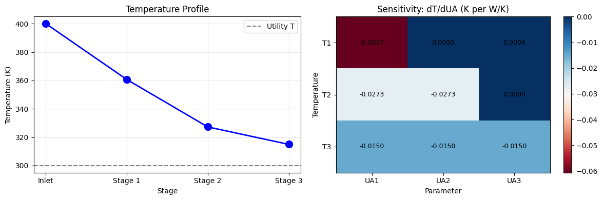
Heat Exchanger Temperature Profile:
  Inlet: 400.0 K
  After stage 1: 360.7 K
  After stage 2: 327.3 K
  After stage 3: 315.0 K
  Outlet: 315.0 K
# Sensitivity of intermediate temperatures to design parameters
def get_temperature_at_stage(params, T_in, stage):
    """Get temperature after a specific stage."""
    _, T_profile = heat_exchanger_stages(params, T_in)
    return T_profile[stage]

# Jacobian: how each intermediate temperature depends on each UA
def temperature_sensitivity_matrix(params, T_in):
    """Compute dT_i/dUA_j for all stages."""
    n_stages = len(params)

    sensitivities = []
    for stage in range(1, n_stages + 1):
        # Gradient of T at this stage w.r.t. all params
        dT_dUA = grad(lambda p: get_temperature_at_stage(p, T_in, stage))(params)
        sensitivities.append(dT_dUA)

    return jnp.array(sensitivities)

sens_matrix = temperature_sensitivity_matrix(params, T_in)

print("\nSensitivity Matrix: dT_i/dUA_j (K per W/K):")
print("=" * 60)
print(f"{'Stage':<10}" + "".join(f"{'dT/dUA'+str(j+1):>15}" for j in range(len(params))))
print("-" * 60)
for i, row in enumerate(sens_matrix):
    print(f"T_{i+1:<8}" + "".join(f"{val:>15.6f}" for val in row))

print("\nInterpretation:")
print("  - Increasing UA1 by 1 W/K decreases T1 by", f"{abs(sens_matrix[0, 0]):.4f} K")
print("  - UA1 has no effect on T2 or T3 (upstream only affects downstream)")
print("  - Actually, all UAs affect downstream temperatures!")
Sensitivity Matrix: dT_i/dUA_j (K per W/K):
============================================================
Stage             dT/dUA1        dT/dUA2        dT/dUA3
------------------------------------------------------------
T_1             -0.060653       0.000000       0.000000
T_2             -0.027253      -0.027253       0.000000
T_3             -0.014957      -0.014957      -0.014957

Interpretation:
  - Increasing UA1 by 1 W/K decreases T1 by 0.0607 K
  - UA1 has no effect on T2 or T3 (upstream only affects downstream)
  - Actually, all UAs affect downstream temperatures!
# Visualize sensitivity
fig, axes = plt.subplots(1, 2, figsize=(12, 4))

# Temperature profile
ax1 = axes[0]
stages = range(len(T_profile))
ax1.plot(stages, T_profile, 'bo-', markersize=10, linewidth=2)
ax1.axhline(300, color='gray', linestyle='--', label='Utility T')
ax1.set_xlabel('Stage')
ax1.set_ylabel('Temperature (K)')
ax1.set_title('Temperature Profile')
ax1.set_xticks(stages)
ax1.set_xticklabels(['Inlet'] + [f'Stage {i+1}' for i in range(len(params))])
ax1.legend()
ax1.grid(True, alpha=0.3)

# Sensitivity heatmap
ax2 = axes[1]
im = ax2.imshow(sens_matrix, cmap='RdBu', aspect='auto')
ax2.set_xticks(range(len(params)))
ax2.set_xticklabels([f'UA{i+1}' for i in range(len(params))])
ax2.set_yticks(range(len(params)))
ax2.set_yticklabels([f'T{i+1}' for i in range(len(params))])
ax2.set_xlabel('Parameter')
ax2.set_ylabel('Temperature')
ax2.set_title('Sensitivity: dT/dUA (K per W/K)')
plt.colorbar(im, ax=ax2)

# Add values
for i in range(len(params)):
    for j in range(len(params)):
        ax2.text(j, i, f'{sens_matrix[i,j]:.4f}', ha='center', va='center', fontsize=9)

plt.tight_layout()
plt.show()
7. Chemical Engineering Example: Reactor Cascade Analysis#
Analyze a cascade of CSTRs where we want derivatives of intermediate concentrations.
def cstr_cascade(params, feed):
    """
    Cascade of CSTRs with first-order reaction A -> B.

    params: dict with 'k' (rate constants), 'V' (volumes), 'T' (temperatures)
    feed: dict with 'C_A0' (feed concentration), 'F' (flow rate)

    Returns: (final_conversion, detailed_results)
    """
    k_values = params['k']
    V_values = params['V']
    T_values = params['T']

    C_A0, F = feed['C_A0'], feed['F']
    E_over_R = 5000.0  # Activation energy / R

    # Track all intermediate values
    results = {
        'C_A': [C_A0],      # Concentrations after each reactor
        'X': [0.0],         # Conversions
        'r': [],            # Reaction rates
        'tau': []           # Residence times
    }

    C_A = C_A0

    for i, (k0, V, T) in enumerate(zip(k_values, V_values, T_values)):
        tau = V / F
        k = k0 * jnp.exp(-E_over_R / T)  # Arrhenius

        # Steady-state CSTR: C_A_out = C_A_in / (1 + k*tau)
        C_A_out = C_A / (1 + k * tau)
        r = k * C_A_out  # Reaction rate
        X = 1 - C_A_out / C_A0  # Overall conversion

        results['C_A'].append(C_A_out)
        results['X'].append(X)
        results['r'].append(r)
        results['tau'].append(tau)

        C_A = C_A_out

    final_conversion = 1 - C_A / C_A0

    # Convert lists to arrays
    results = {k: jnp.array(v) for k, v in results.items()}

    return final_conversion, results

# System setup: 3 CSTRs in series
params = {
    'k': jnp.array([1e5, 1e5, 1e5]),       # Pre-exponential factors
    'V': jnp.array([10.0, 15.0, 20.0]),    # Volumes (m³)
    'T': jnp.array([350.0, 360.0, 370.0])  # Temperatures (K)
}
feed = {'C_A0': jnp.array(1.0), 'F': jnp.array(1.0)}  # mol/m³, m³/s

conversion, results = cstr_cascade(params, feed)

print("CSTR Cascade Results:")
print("=" * 60)
print(f"\nConcentration profile (mol/m³):")
for i, C in enumerate(results['C_A']):
    label = 'Feed' if i == 0 else f'After CSTR {i}'
    print(f"  {label}: C_A = {C:.4f}")

print(f"\nConversion profile:")
for i, X in enumerate(results['X']):
    if i > 0:
        print(f"  After CSTR {i}: X = {X:.4f} ({X*100:.1f}%)")

print(f"\nFinal conversion: {conversion:.4f} ({conversion*100:.1f}%)")
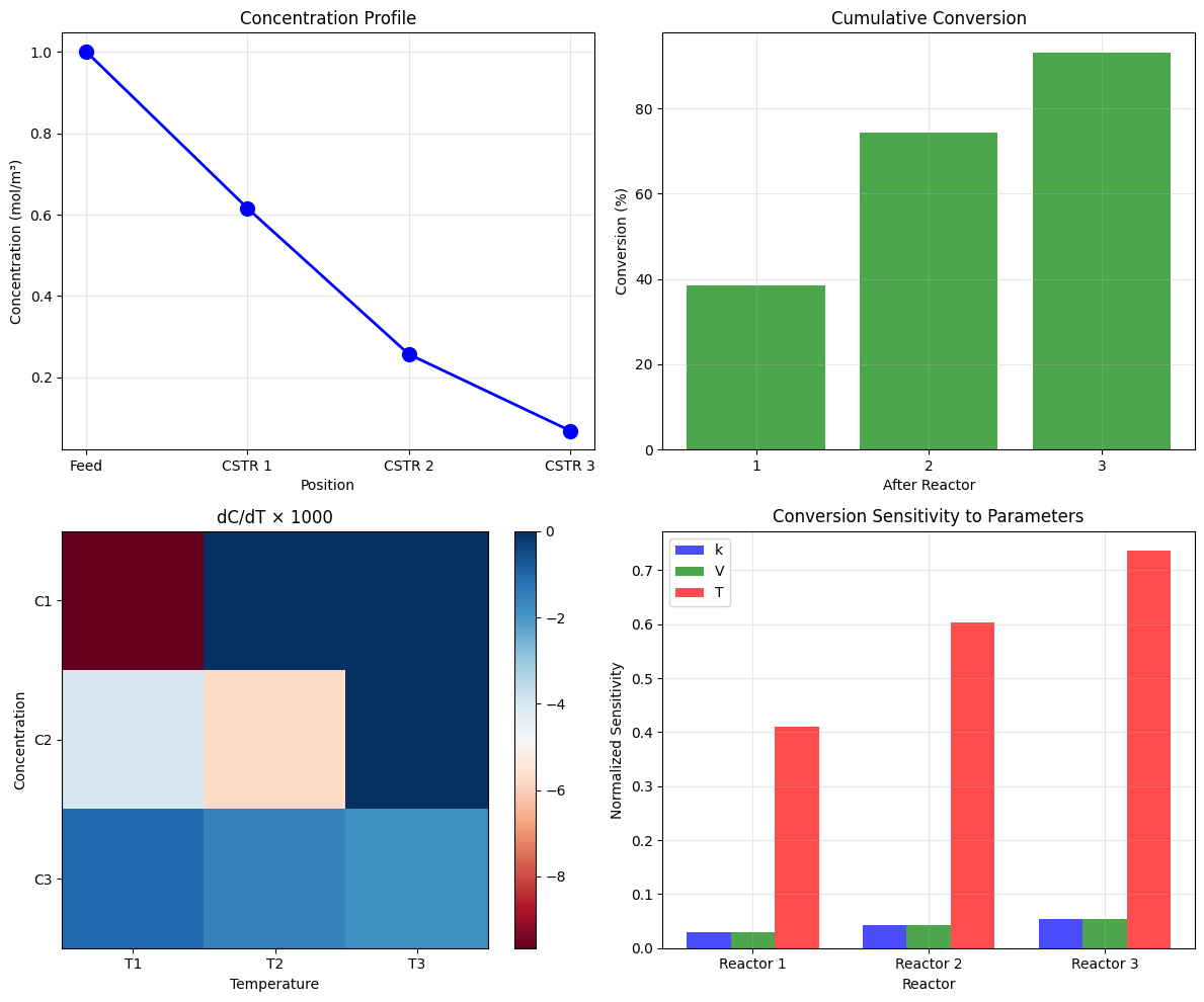
CSTR Cascade Results:
============================================================

Concentration profile (mol/m³):
  Feed: C_A = 1.0000
  After CSTR 1: C_A = 0.6154
  After CSTR 2: C_A = 0.2571
  After CSTR 3: C_A = 0.0694

Conversion profile:
  After CSTR 1: X = 0.3846 (38.5%)
  After CSTR 2: X = 0.7429 (74.3%)
  After CSTR 3: X = 0.9306 (93.1%)

Final conversion: 0.9306 (93.1%)
# Sensitivity analysis: How do intermediate concentrations depend on temperatures?

def concentration_after_reactor(params, feed, reactor_idx):
    """Get concentration after a specific reactor."""
    _, results = cstr_cascade(params, feed)
    return results['C_A'][reactor_idx + 1]  # +1 because index 0 is feed

def compute_sensitivity_to_temperature(params, feed):
    """Compute dC_A_i / dT_j for all reactor pairs."""
    n_reactors = len(params['T'])

    sensitivity = jnp.zeros((n_reactors, n_reactors))

    for i in range(n_reactors):
        # Gradient of C_A after reactor i w.r.t. all temperatures
        def get_C_i(T_array):
            params_modified = {**params, 'T': T_array}
            return concentration_after_reactor(params_modified, feed, i)

        dC_dT = grad(get_C_i)(params['T'])
        sensitivity = sensitivity.at[i, :].set(dC_dT)

    return sensitivity

sens_T = compute_sensitivity_to_temperature(params, feed)

print("\nSensitivity: dC_A_i / dT_j (mol/m³ per K):")
print("=" * 60)
print(f"{'Conc.':<10}" + "".join(f"{'dC/dT'+str(j+1):>15}" for j in range(len(params['T']))))
print("-" * 60)
for i in range(len(params['T'])):
    print(f"C_A_{i+1:<6}" + "".join(f"{sens_T[i,j]:>15.6f}" for j in range(len(params['T']))))

print("\nKey insights:")
print("  - Negative values: higher T -> lower C_A (more reaction)")
print("  - Upper triangular structure: upstream T affects downstream C")
print("  - Diagonal dominance: each reactor most sensitive to its own T")
Sensitivity: dC_A_i / dT_j (mol/m³ per K):
============================================================
Conc.              dC/dT1         dC/dT2         dC/dT3
------------------------------------------------------------
C_A_1           -0.009660       0.000000       0.000000
C_A_2           -0.004035      -0.005775       0.000000
C_A_3           -0.001089      -0.001559      -0.001850

Key insights:
  - Negative values: higher T -> lower C_A (more reaction)
  - Upper triangular structure: upstream T affects downstream C
  - Diagonal dominance: each reactor most sensitive to its own T
# Full sensitivity analysis: gradient of conversion and all intermediates
# w.r.t. all design parameters

def full_sensitivity_analysis(params, feed):
    """
    Compute sensitivities of all outputs to all inputs.
    """
    # Flatten parameters for easier differentiation
    n = len(params['T'])

    # Sensitivity of final conversion
    def get_conversion(p_flat):
        p = {'k': p_flat[:n], 'V': p_flat[n:2*n], 'T': p_flat[2*n:]}
        conv, _ = cstr_cascade(p, feed)
        return conv

    p_flat = jnp.concatenate([params['k'], params['V'], params['T']])

    # Gradient of conversion
    grad_conversion = grad(get_conversion)(p_flat)

    # Normalized sensitivities
    conv_value = get_conversion(p_flat)
    norm_sens = (p_flat / conv_value) * grad_conversion

    return {
        'grad_k': grad_conversion[:n],
        'grad_V': grad_conversion[n:2*n],
        'grad_T': grad_conversion[2*n:],
        'norm_k': norm_sens[:n],
        'norm_V': norm_sens[n:2*n],
        'norm_T': norm_sens[2*n:]
    }

sens = full_sensitivity_analysis(params, feed)

print("\nConversion Sensitivity Analysis:")
print("=" * 60)
print(f"\n{'Parameter':<10} {'dX/dp':<15} {'Normalized':<15} {'Interpretation'}")
print("-" * 60)

param_names = ['k1', 'k2', 'k3', 'V1', 'V2', 'V3', 'T1', 'T2', 'T3']
all_grads = jnp.concatenate([sens['grad_k'], sens['grad_V'], sens['grad_T']])
all_norms = jnp.concatenate([sens['norm_k'], sens['norm_V'], sens['norm_T']])

for name, g, n in zip(param_names, all_grads, all_norms):
    direction = "↑" if g > 0 else "↓" if g < 0 else "—"
    print(f"{name:<10} {g:<15.6f} {n:<15.4f} {direction} conversion")
Conversion Sensitivity Analysis:
============================================================

Parameter  dX/dp           Normalized      Interpretation
------------------------------------------------------------
k1         0.000000        0.0287          ↑ conversion
k2         0.000000        0.0434          ↑ conversion
k3         0.000001        0.0544          ↑ conversion
V1         0.002668        0.0287          ↑ conversion
V2         0.002693        0.0434          ↑ conversion
V3         0.002533        0.0544          ↑ conversion
T1         0.001089        0.4096          ↑ conversion
T2         0.001559        0.6030          ↑ conversion
T3         0.001850        0.7356          ↑ conversion
# Visualize the cascade and sensitivities
fig, axes = plt.subplots(2, 2, figsize=(12, 10))

# Plot 1: Concentration profile
ax1 = axes[0, 0]
reactor_positions = range(len(results['C_A']))
ax1.plot(reactor_positions, results['C_A'], 'bo-', markersize=10, linewidth=2)
ax1.set_xlabel('Position')
ax1.set_ylabel('Concentration (mol/m³)')
ax1.set_title('Concentration Profile')
ax1.set_xticks(reactor_positions)
ax1.set_xticklabels(['Feed'] + [f'CSTR {i+1}' for i in range(len(params['T']))])
ax1.grid(True, alpha=0.3)

# Plot 2: Conversion profile
ax2 = axes[0, 1]
ax2.bar(range(1, len(results['X'])), results['X'][1:] * 100, color='green', alpha=0.7)
ax2.set_xlabel('After Reactor')
ax2.set_ylabel('Conversion (%)')
ax2.set_title('Cumulative Conversion')
ax2.set_xticks(range(1, len(results['X'])))
ax2.grid(True, alpha=0.3)

# Plot 3: Sensitivity heatmap (concentration to temperature)
ax3 = axes[1, 0]
im = ax3.imshow(sens_T * 1000, cmap='RdBu', aspect='auto')  # Scale for visibility
ax3.set_xticks(range(len(params['T'])))
ax3.set_xticklabels([f'T{i+1}' for i in range(len(params['T']))])
ax3.set_yticks(range(len(params['T'])))
ax3.set_yticklabels([f'C{i+1}' for i in range(len(params['T']))])
ax3.set_xlabel('Temperature')
ax3.set_ylabel('Concentration')
ax3.set_title('dC/dT × 1000')
plt.colorbar(im, ax=ax3)

# Plot 4: Normalized sensitivities bar chart
ax4 = axes[1, 1]
width = 0.25
x = jnp.arange(len(params['T']))
ax4.bar(x - width, sens['norm_k'], width, label='k', color='blue', alpha=0.7)
ax4.bar(x, sens['norm_V'], width, label='V', color='green', alpha=0.7)
ax4.bar(x + width, sens['norm_T'], width, label='T', color='red', alpha=0.7)
ax4.set_xlabel('Reactor')
ax4.set_ylabel('Normalized Sensitivity')
ax4.set_title('Conversion Sensitivity to Parameters')
ax4.set_xticks(x)
ax4.set_xticklabels([f'Reactor {i+1}' for i in range(len(params['T']))])
ax4.legend()
ax4.grid(True, alpha=0.3)

plt.tight_layout()
plt.show()
Summary#
This tutorial covered techniques for accessing intermediate derivatives:
Technique |
Use Case |
Code Pattern |
|---|---|---|
|
Return intermediates during grad |
|
|
Get value + gradient efficiently |
|
|
Jacobian of intermediate |
|
Custom VJP |
Full control over backward pass |
|
Structured output |
Return intermediates as dict |
|
Key Takeaways#
Structure functions to expose intermediates: Return
(output, aux_dict)from the startUse
has_aux=True: JAX only differentiates through the first outputJacobians for vector intermediates: Use
jacobian()for multi-dimensional sensitivityCustom VJP for full control: Can track/return gradient at any intermediate
Engineering insight: Intermediate sensitivities reveal which parameters matter where
Chemical Engineering Applications#
Reactor cascades: How does conversion at each stage depend on operating conditions?
Heat exchanger networks: Temperature sensitivity at each point
Distillation columns: Composition profile sensitivity to reflux ratio
Control systems: How do intermediate states respond to inputs?