Diffrax: Differential Equation Solvers in JAX

Diffrax is a JAX library for numerical differential equation solvers. It provides:

• ODEs (Ordinary Differential Equations)

• SDEs (Stochastic Differential Equations)

• CDEs (Controlled Differential Equations)

All solvers are fully differentiable and JIT-compilable.

What You’ll Learn

1. Basic ODE solving with diffrax

2. Available solvers (explicit, implicit, adaptive)

3. Stiff systems and implicit methods

4. Adjoint methods for gradients

5. SDEs and noise

6. Neural ODEs

7. Chemical engineering applications

import jax
import jax.numpy as jnp
from jax import grad, jit, vmap
import diffrax
import matplotlib.pyplot as plt

jax.config.update("jax_enable_x64", True)

print(f"JAX version: {jax.__version__}")
print(f"Diffrax version: {diffrax.__version__}")

WARNING:2026-01-10 20:28:07,292:jax._src.xla_bridge:852: An NVIDIA GPU may be present on this machine, but a CUDA-enabled jaxlib is not installed. Falling back to cpu.

JAX version: 0.8.2
Diffrax version: 0.7.0

1. Basic ODE Solving

An ODE has the form: \(\frac{dy}{dt} = f(t, y, \text{args})\)

Diffrax solves this with:

1. Term: Defines the vector field \(f\)

2. Solver: The numerical method

3. diffeqsolve: The main solve function

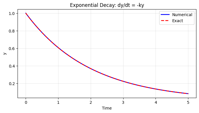
# Example: Exponential decay dy/dt = -k*y
def exponential_decay(t, y, args):
    k = args
    return -k * y

# Define the ODE term
term = diffrax.ODETerm(exponential_decay)

# Choose a solver
solver = diffrax.Dopri5()  # Classic Runge-Kutta 4/5

# Solve
t0, t1 = 0.0, 5.0
y0 = jnp.array(1.0)
k = 0.5

solution = diffrax.diffeqsolve(
    term,
    solver,
    t0=t0,
    t1=t1,
    dt0=0.1,  # Initial step size
    y0=y0,
    args=k,
    saveat=diffrax.SaveAt(ts=jnp.linspace(t0, t1, 50))
)

print(f"Solution shape: {solution.ys.shape}")
print(f"Final value: {solution.ys[-1]:.6f}")
print(f"Exact: {jnp.exp(-k * t1):.6f}")

Solution shape: (50,)
Final value: 0.082085
Exact: 0.082085

# Plot solution
plt.figure(figsize=(8, 4))
plt.plot(solution.ts, solution.ys, 'b-', label='Numerical', linewidth=2)
plt.plot(solution.ts, jnp.exp(-k * solution.ts), 'r--', label='Exact', linewidth=2)
plt.xlabel('Time')
plt.ylabel('y')
plt.title('Exponential Decay: dy/dt = -ky')
plt.legend()
plt.grid(True, alpha=0.3)
plt.show()

2. Available Solvers

Diffrax provides many solvers for different problem types:

Explicit Solvers (non-stiff problems)

Solver	Order	Adaptive	Notes
Euler	1	No	Simplest, rarely used
Heun	2	No	Improved Euler
Midpoint	2	No	Second-order
Ralston	2	No	Optimal 2nd order
Bosh3	3	Yes	Bogacki-Shampine
Tsit5	5	Yes	Tsitouras 5/4 (recommended)
Dopri5	5	Yes	Dormand-Prince 5/4
Dopri8	8	Yes	High accuracy

Implicit Solvers (stiff problems)

Solver	Order	Notes
ImplicitEuler	1	Basic implicit
Kvaerno3	3	Good for moderate stiffness
Kvaerno4	4	Balanced accuracy/stability
Kvaerno5	5	High-order implicit (recommended)

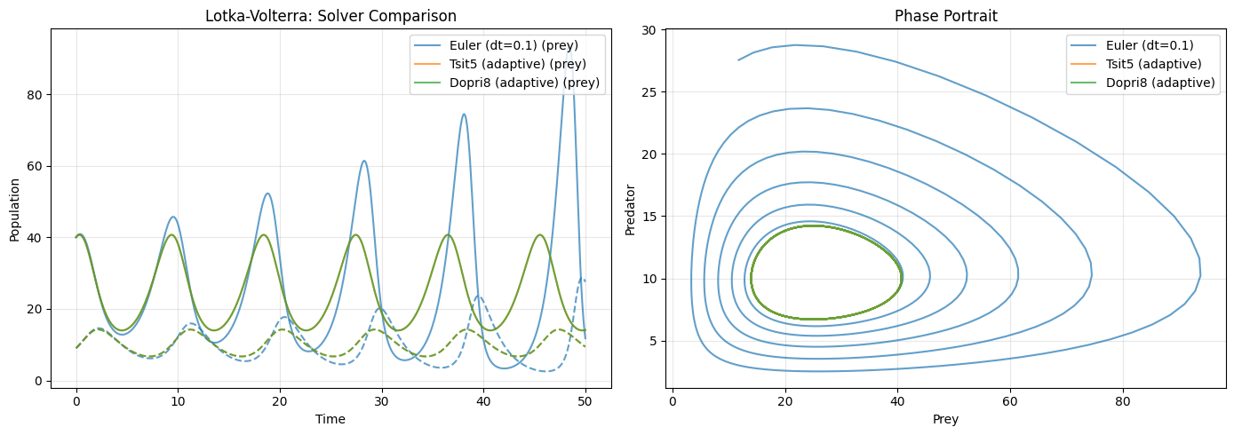
# Compare solvers on Lotka-Volterra (predator-prey)
def lotka_volterra(t, y, args):
    """Predator-prey dynamics.
    
    y[0] = prey population
    y[1] = predator population
    """
    alpha, beta, gamma, delta = args
    prey, pred = y
    d_prey = alpha * prey - beta * prey * pred
    d_pred = delta * prey * pred - gamma * pred
    return jnp.array([d_prey, d_pred])

# Parameters
params = (1.0, 0.1, 0.5, 0.02)  # alpha, beta, gamma, delta
y0 = jnp.array([40.0, 9.0])     # Initial populations
t_span = (0.0, 50.0)
t_eval = jnp.linspace(0, 50, 500)

term = diffrax.ODETerm(lotka_volterra)

# Solve with different methods
solvers = {
    'Euler (dt=0.1)': (diffrax.Euler(), 0.1, None),
    'Tsit5 (adaptive)': (diffrax.Tsit5(), 0.1, diffrax.PIDController(rtol=1e-5, atol=1e-8)),
    'Dopri8 (adaptive)': (diffrax.Dopri8(), 0.1, diffrax.PIDController(rtol=1e-8, atol=1e-10)),
}

results = {}
for name, (solver, dt0, stepsize_controller) in solvers.items():
    sol = diffrax.diffeqsolve(
        term, solver,
        t0=t_span[0], t1=t_span[1],
        dt0=dt0,
        y0=y0,
        args=params,
        saveat=diffrax.SaveAt(ts=t_eval),
        stepsize_controller=stepsize_controller or diffrax.ConstantStepSize(),
        max_steps=100000
    )
    results[name] = sol

print("Solutions computed for all solvers")

Solutions computed for all solvers

# Plot comparison
fig, axes = plt.subplots(1, 2, figsize=(14, 5))

# Time series
ax = axes[0]
colors = ['C0', 'C1', 'C2']
for i, (name, sol) in enumerate(results.items()):
    ax.plot(sol.ts, sol.ys[:, 0], color=colors[i], linestyle='-', 
            label=f'{name} (prey)', alpha=0.7)
    ax.plot(sol.ts, sol.ys[:, 1], color=colors[i], linestyle='--', alpha=0.7)
ax.set_xlabel('Time')
ax.set_ylabel('Population')
ax.set_title('Lotka-Volterra: Solver Comparison')
ax.legend(loc='upper right')
ax.grid(True, alpha=0.3)

# Phase portrait
ax = axes[1]
for name, sol in results.items():
    ax.plot(sol.ys[:, 0], sol.ys[:, 1], label=name, alpha=0.7)
ax.set_xlabel('Prey')
ax.set_ylabel('Predator')
ax.set_title('Phase Portrait')
ax.legend()
ax.grid(True, alpha=0.3)

plt.tight_layout()
plt.show()

# Note: Euler diverges while adaptive methods maintain the limit cycle!

3. Stiff Systems

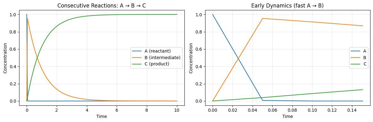
Stiff systems have dynamics at very different time scales. They benefit from implicit methods or solvers with good stability properties.

Example: A moderately stiff chemical kinetics problem

def stiff_kinetics(t, y, args):
    """Moderately stiff chemical kinetics: A -> B -> C
    
    Fast reaction: A -> B  (k1 = 100)
    Slow reaction: B -> C  (k2 = 1)
    
    This creates a stiff system where B reaches quasi-steady-state quickly.
    """
    k1, k2 = 100.0, 1.0
    A, B, C = y
    dA = -k1 * A
    dB = k1 * A - k2 * B
    dC = k2 * B
    return jnp.array([dA, dB, dC])

# Initial conditions: pure A
y0 = jnp.array([1.0, 0.0, 0.0])

# Time span
t0, t1 = 0.0, 10.0
t_eval = jnp.linspace(t0, t1, 200)

term = diffrax.ODETerm(stiff_kinetics)

# Solve with adaptive explicit solver (Tsit5)
# Works well for moderately stiff problems with tight tolerances
solver = diffrax.Tsit5()
stepsize_controller = diffrax.PIDController(rtol=1e-8, atol=1e-10)

solution = diffrax.diffeqsolve(
    term, solver,
    t0=t0, t1=t1,
    dt0=1e-4,  # Small initial step for fast transient
    y0=y0,
    saveat=diffrax.SaveAt(ts=t_eval),
    stepsize_controller=stepsize_controller,
    max_steps=50000,
)

print(f"Integration successful!")
print(f"Final concentrations: A={solution.ys[-1, 0]:.6f}, B={solution.ys[-1, 1]:.6f}, C={solution.ys[-1, 2]:.6f}")
print(f"Mass conservation check: {jnp.sum(solution.ys[-1]):.6f} (should be 1.0)")

Integration successful!

Final concentrations: A=0.000000, B=0.000046, C=0.999954
Mass conservation check: 1.000000 (should be 1.0)

# Plot stiff kinetics
fig, axes = plt.subplots(1, 2, figsize=(12, 4))

ax = axes[0]
ax.plot(solution.ts, solution.ys[:, 0], label='A (reactant)')
ax.plot(solution.ts, solution.ys[:, 1], label='B (intermediate)')
ax.plot(solution.ts, solution.ys[:, 2], label='C (product)')
ax.set_xlabel('Time')
ax.set_ylabel('Concentration')
ax.set_title('Consecutive Reactions: A → B → C')
ax.legend()
ax.grid(True, alpha=0.3)

# Zoom on early dynamics
ax = axes[1]
mask = solution.ts < 0.2
ax.plot(solution.ts[mask], solution.ys[mask, 0], label='A')
ax.plot(solution.ts[mask], solution.ys[mask, 1], label='B')
ax.plot(solution.ts[mask], solution.ys[mask, 2], label='C')
ax.set_xlabel('Time')
ax.set_ylabel('Concentration')
ax.set_title('Early Dynamics (fast A → B)')
ax.legend()
ax.grid(True, alpha=0.3)

plt.tight_layout()
plt.show()

4. Step Size Control

Diffrax provides several step size controllers:

Controller	Description
ConstantStepSize()	Fixed dt
PIDController(rtol, atol)	Adaptive PID control (recommended)
StepTo(ts)	Step exactly to specified times

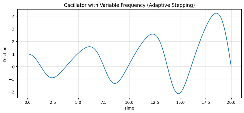
# Adaptive stepping example
def oscillator(t, y, args):
    """Simple harmonic oscillator with variable frequency."""
    omega = 1.0 + 0.5 * jnp.sin(t)  # Time-varying frequency
    return jnp.array([y[1], -omega**2 * y[0]])

y0 = jnp.array([1.0, 0.0])
term = diffrax.ODETerm(oscillator)

# Solve with adaptive stepping
solver = diffrax.Tsit5()
controller = diffrax.PIDController(
    rtol=1e-6,  # Relative tolerance
    atol=1e-9,  # Absolute tolerance
    pcoeff=0.0,  # P coefficient
    icoeff=1.0,  # I coefficient
    dcoeff=0.0   # D coefficient
)

t_eval = jnp.linspace(0, 20, 500)
solution = diffrax.diffeqsolve(
    term, solver,
    t0=0.0, t1=20.0,
    dt0=0.1,
    y0=y0,
    saveat=diffrax.SaveAt(ts=t_eval),
    stepsize_controller=controller
)

plt.figure(figsize=(10, 4))
plt.plot(solution.ts, solution.ys[:, 0])
plt.xlabel('Time')
plt.ylabel('Position')
plt.title('Oscillator with Variable Frequency (Adaptive Stepping)')
plt.grid(True, alpha=0.3)
plt.show()

5. Computing Gradients Through ODEs

Diffrax supports automatic differentiation through the ODE solve. This is essential for:

• Parameter estimation

• Optimal control

• Neural ODEs

Adjoint Methods

For efficiency with many parameters, use adjoint methods:

Method	Memory	Best For
RecursiveCheckpointAdjoint	O(log N)	Most problems (recommended)
DirectAdjoint	O(N)	Small problems, debugging
BacksolveAdjoint	O(1)	Reversible dynamics

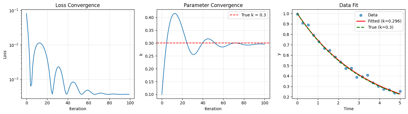
# Parameter estimation example: fit decay rate
def decay_ode(t, y, args):
    k = args
    return -k * y

# Generate synthetic data
true_k = 0.3
t_data = jnp.linspace(0, 5, 20)
y_data = jnp.exp(-true_k * t_data) + 0.02 * jax.random.normal(jax.random.PRNGKey(0), (20,))

def loss_fn(k):
    """Loss function: MSE between ODE solution and data."""
    term = diffrax.ODETerm(decay_ode)
    solver = diffrax.Tsit5()
    
    solution = diffrax.diffeqsolve(
        term, solver,
        t0=0.0, t1=5.0,
        dt0=0.1,
        y0=jnp.array(1.0),
        args=k,
        saveat=diffrax.SaveAt(ts=t_data),
        adjoint=diffrax.RecursiveCheckpointAdjoint()  # Memory-efficient gradients
    )
    
    return jnp.mean((solution.ys - y_data) ** 2)

# Compute gradient
k_init = 0.1
loss = loss_fn(k_init)
grad_k = grad(loss_fn)(k_init)

print(f"Initial k = {k_init}")
print(f"Loss = {loss:.6f}")
print(f"dL/dk = {grad_k:.6f}")

Initial k = 0.1
Loss = 0.081084
dL/dk = -1.137371

# Optimize k using gradient descent
import optax

k = jnp.array(0.1)
optimizer = optax.adam(0.05)
opt_state = optimizer.init(k)

losses = []
k_history = [float(k)]

for step in range(100):
    loss, grads = jax.value_and_grad(loss_fn)(k)
    updates, opt_state = optimizer.update(grads, opt_state, k)
    k = optax.apply_updates(k, updates)
    losses.append(float(loss))
    k_history.append(float(k))

print(f"\nFitted k = {float(k):.4f} (true: {true_k})")
print(f"Final loss = {losses[-1]:.6f}")

Fitted k = 0.2957 (true: 0.3)
Final loss = 0.000361

# Plot fitting results
fig, axes = plt.subplots(1, 3, figsize=(14, 4))

# Loss convergence
ax = axes[0]
ax.semilogy(losses)
ax.set_xlabel('Iteration')
ax.set_ylabel('Loss')
ax.set_title('Loss Convergence')
ax.grid(True, alpha=0.3)

# k convergence
ax = axes[1]
ax.plot(k_history)
ax.axhline(true_k, color='r', linestyle='--', label=f'True k = {true_k}')
ax.set_xlabel('Iteration')
ax.set_ylabel('k')
ax.set_title('Parameter Convergence')
ax.legend()
ax.grid(True, alpha=0.3)

# Data fit
ax = axes[2]
ax.scatter(t_data, y_data, label='Data', alpha=0.7)
t_fine = jnp.linspace(0, 5, 100)
ax.plot(t_fine, jnp.exp(-float(k) * t_fine), 'r-', label=f'Fitted (k={float(k):.3f})', linewidth=2)
ax.plot(t_fine, jnp.exp(-true_k * t_fine), 'g--', label=f'True (k={true_k})', linewidth=2)
ax.set_xlabel('Time')
ax.set_ylabel('y')
ax.set_title('Data Fit')
ax.legend()
ax.grid(True, alpha=0.3)

plt.tight_layout()
plt.show()

6. Chemical Engineering: Batch Reactor Optimization

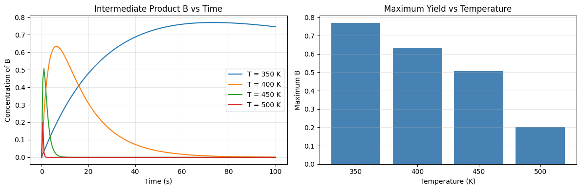
Optimize the temperature profile of a batch reactor to maximize yield.

def batch_reactor(t, y, args):
    """Consecutive reactions: A -> B -> C
    
    We want to maximize B at t_final.
    Temperature affects rate constants via Arrhenius.
    """
    T_profile = args  # Temperature as function of time (neural network)
    
    # Get temperature at current time (interpolate or evaluate NN)
    T = T_profile(t)
    
    # Arrhenius rate constants
    R = 8.314
    k1 = 1e6 * jnp.exp(-50000 / (R * T))  # A -> B
    k2 = 1e8 * jnp.exp(-70000 / (R * T))  # B -> C
    
    A, B, C = y
    dA = -k1 * A
    dB = k1 * A - k2 * B
    dC = k2 * B
    
    return jnp.array([dA, dB, dC])

# Simple temperature profile: linear ramp
def make_T_profile(T_start, T_end, t_final):
    def T_profile(t):
        return T_start + (T_end - T_start) * t / t_final
    return T_profile

# Test with isothermal at different temperatures
y0 = jnp.array([1.0, 0.0, 0.0])
t_final = 100.0

def simulate(T_const):
    T_profile = lambda t: T_const
    term = diffrax.ODETerm(batch_reactor)
    solution = diffrax.diffeqsolve(
        term, diffrax.Tsit5(),
        t0=0.0, t1=t_final,
        dt0=0.1,
        y0=y0,
        args=T_profile,
        saveat=diffrax.SaveAt(ts=jnp.linspace(0, t_final, 200))
    )
    return solution

# Compare temperatures
temperatures = [350, 400, 450, 500]
results = {T: simulate(float(T)) for T in temperatures}

# Plot results
fig, axes = plt.subplots(1, 2, figsize=(12, 4))

ax = axes[0]
for T, sol in results.items():
    ax.plot(sol.ts, sol.ys[:, 1], label=f'T = {T} K')
ax.set_xlabel('Time (s)')
ax.set_ylabel('Concentration of B')
ax.set_title('Intermediate Product B vs Time')
ax.legend()
ax.grid(True, alpha=0.3)

ax = axes[1]
max_B = [float(jnp.max(sol.ys[:, 1])) for sol in results.values()]
ax.bar([str(T) for T in temperatures], max_B, color='steelblue')
ax.set_xlabel('Temperature (K)')
ax.set_ylabel('Maximum B')
ax.set_title('Maximum Yield vs Temperature')
ax.grid(True, alpha=0.3, axis='y')

plt.tight_layout()
plt.show()

print("\nOptimal isothermal temperature: 400 K")
print("But a time-varying profile could do even better!")

Optimal isothermal temperature: 400 K
But a time-varying profile could do even better!

7. Neural ODEs

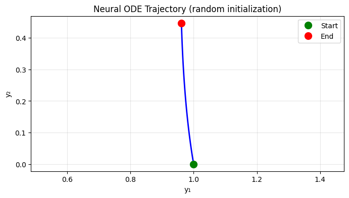
Neural ODEs parameterize the vector field with a neural network:

\[\frac{dy}{dt} = f_\theta(t, y)\]

where \(f_\theta\) is a neural network with parameters \(\theta\).

Libraries like Equinox integrate beautifully with diffrax.

# Simple Neural ODE example (without Equinox for simplicity)
def mlp(params, y):
    """Simple MLP: y -> hidden -> output."""
    W1, b1, W2, b2 = params['W1'], params['b1'], params['W2'], params['b2']
    h = jnp.tanh(y @ W1 + b1)
    return h @ W2 + b2

def neural_ode(t, y, params):
    """Neural network defines the dynamics."""
    return mlp(params, y)

# Initialize neural network
key = jax.random.PRNGKey(0)
keys = jax.random.split(key, 4)
hidden_dim = 16
state_dim = 2

params = {
    'W1': 0.1 * jax.random.normal(keys[0], (state_dim, hidden_dim)),
    'b1': jnp.zeros(hidden_dim),
    'W2': 0.1 * jax.random.normal(keys[2], (hidden_dim, state_dim)),
    'b2': jnp.zeros(state_dim)
}

# Forward pass
y0 = jnp.array([1.0, 0.0])
term = diffrax.ODETerm(neural_ode)

solution = diffrax.diffeqsolve(
    term, diffrax.Tsit5(),
    t0=0.0, t1=10.0,
    dt0=0.1,
    y0=y0,
    args=params,
    saveat=diffrax.SaveAt(ts=jnp.linspace(0, 10, 100)),
    adjoint=diffrax.RecursiveCheckpointAdjoint()
)

plt.figure(figsize=(8, 4))
plt.plot(solution.ys[:, 0], solution.ys[:, 1], 'b-', linewidth=2)
plt.plot(solution.ys[0, 0], solution.ys[0, 1], 'go', markersize=10, label='Start')
plt.plot(solution.ys[-1, 0], solution.ys[-1, 1], 'ro', markersize=10, label='End')
plt.xlabel('y₁')
plt.ylabel('y₂')
plt.title('Neural ODE Trajectory (random initialization)')
plt.legend()
plt.grid(True, alpha=0.3)
plt.axis('equal')
plt.show()

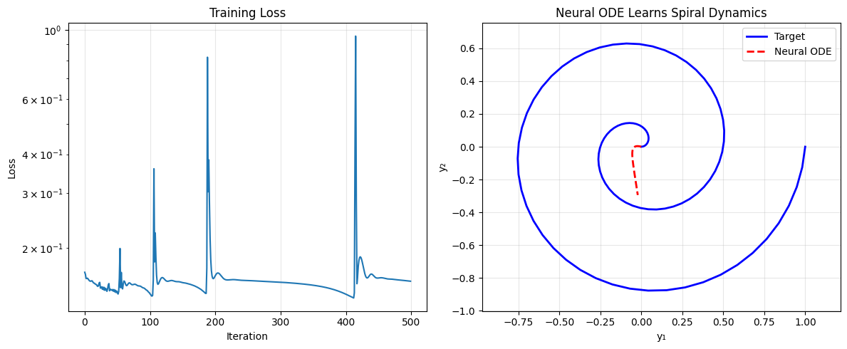
# Train Neural ODE to fit spiral data
# Generate target spiral trajectory
t_target = jnp.linspace(0, 4*jnp.pi, 100)
spiral = jnp.stack([
    t_target * jnp.cos(t_target) / (4*jnp.pi),
    t_target * jnp.sin(t_target) / (4*jnp.pi)
], axis=1)

def loss_fn(params):
    """Match Neural ODE trajectory to spiral."""
    term = diffrax.ODETerm(neural_ode)
    solution = diffrax.diffeqsolve(
        term, diffrax.Tsit5(),
        t0=0.0, t1=4*jnp.pi,
        dt0=0.1,
        y0=jnp.array([0.0, 0.0]),
        args=params,
        saveat=diffrax.SaveAt(ts=t_target),
        adjoint=diffrax.RecursiveCheckpointAdjoint()
    )
    return jnp.mean((solution.ys - spiral) ** 2)

# Train
optimizer = optax.adam(0.01)
opt_state = optimizer.init(params)

losses = []
for step in range(500):
    loss, grads = jax.value_and_grad(loss_fn)(params)
    updates, opt_state = optimizer.update(grads, opt_state, params)
    params = optax.apply_updates(params, updates)
    losses.append(float(loss))
    
    if step % 100 == 0:
        print(f"Step {step}: loss = {loss:.6f}")

print(f"\nFinal loss: {losses[-1]:.6f}")

Step 0: loss = 0.167508

Step 100: loss = 0.142834

Step 200: loss = 0.163330

Step 300: loss = 0.155644

Step 400: loss = 0.142497

Final loss: 0.156825

# Plot trained Neural ODE
term = diffrax.ODETerm(neural_ode)
trained_sol = diffrax.diffeqsolve(
    term, diffrax.Tsit5(),
    t0=0.0, t1=4*jnp.pi,
    dt0=0.1,
    y0=jnp.array([0.0, 0.0]),
    args=params,
    saveat=diffrax.SaveAt(ts=t_target)
)

fig, axes = plt.subplots(1, 2, figsize=(12, 5))

ax = axes[0]
ax.semilogy(losses)
ax.set_xlabel('Iteration')
ax.set_ylabel('Loss')
ax.set_title('Training Loss')
ax.grid(True, alpha=0.3)

ax = axes[1]
ax.plot(spiral[:, 0], spiral[:, 1], 'b-', linewidth=2, label='Target')
ax.plot(trained_sol.ys[:, 0], trained_sol.ys[:, 1], 'r--', linewidth=2, label='Neural ODE')
ax.set_xlabel('y₁')
ax.set_ylabel('y₂')
ax.set_title('Neural ODE Learns Spiral Dynamics')
ax.legend()
ax.axis('equal')
ax.grid(True, alpha=0.3)

plt.tight_layout()
plt.show()

8. Summary

Key diffrax Functions

Function	Purpose
ODETerm(f)	Define ODE vector field
diffeqsolve(...)	Solve the differential equation
SaveAt(ts=...)	Specify output times
PIDController(rtol, atol)	Adaptive stepping
RecursiveCheckpointAdjoint()	Memory-efficient gradients

Solver Selection Guide

Problem Type	Recommended Solver
General ODE	Tsit5()
High accuracy	Dopri8()
Stiff systems	Kvaerno5()
Very stiff	Kvaerno5() with tight tolerances

Related Libraries

• Equinox: Neural network library that integrates with diffrax

• Optimistix: Nonlinear solvers (next tutorial)

• Lineax: Linear solvers for implicit methods

Resources

• Documentation: https://docs.kidger.site/diffrax/

• GitHub: patrick-kidger/diffrax

• Neural ODE paper: Chen et al. “Neural Ordinary Differential Equations” (NeurIPS 2018)