Gaussian Processes in JAX with GPJax

Gaussian Processes (GPs) are powerful probabilistic models that provide:

• Predictions with uncertainty estimates

• Flexible nonparametric modeling

• Principled Bayesian inference

GPJax is a didactic GP library built on JAX.

What You’ll Learn

1. GP fundamentals: prior, posterior, prediction

2. Kernel functions (covariance functions)

3. Kernel composition and design

4. Hyperparameter optimization

5. Sparse GPs for large datasets

6. Chemical engineering applications

import os
os.environ['JAX_PLATFORMS'] = 'cpu'  # Force CPU to avoid Metal backend issues

import jax
import jax.numpy as jnp
from jax import random
import matplotlib.pyplot as plt
import optax

jax.config.update("jax_enable_x64", True)

# GPJax imports
import gpjax as gpx
from gpjax.kernels import (
    RBF, Matern12, Matern32, Matern52,
    Polynomial, Periodic, Linear,
    SumKernel, ProductKernel
)

print(f"JAX version: {jax.__version__}")
print(f"GPJax version: {gpx.__version__}")

JAX version: 0.8.2
GPJax version: 0.13.4

---

Part 1: GP Fundamentals

A Gaussian Process is a collection of random variables, any finite number of which have a joint Gaussian distribution.

\[f(x) \sim \mathcal{GP}(m(x), k(x, x'))\]

• \(m(x)\): Mean function (often zero)

• \(k(x, x')\): Covariance/kernel function

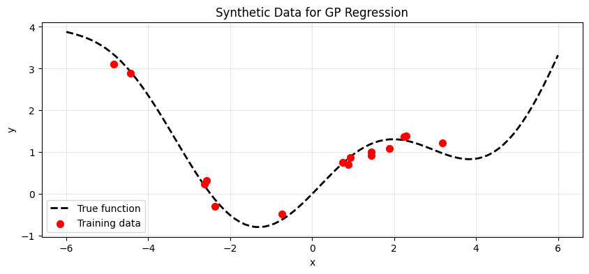
# Generate synthetic data
key = random.PRNGKey(42)

# True function: f(x) = sin(x) + 0.1*x^2
def true_function(x):
    return jnp.sin(x) + 0.1 * x**2

# Training data
n_train = 15
X_train = random.uniform(key, (n_train, 1), minval=-5, maxval=5)
X_train = jnp.sort(X_train, axis=0)  # Sort for visualization
noise_std = 0.2
y_train = true_function(X_train) + noise_std * random.normal(random.PRNGKey(1), X_train.shape)

# Test points
X_test = jnp.linspace(-6, 6, 100)[:, None]

# Plot data
plt.figure(figsize=(10, 4))
plt.plot(X_test, true_function(X_test), 'k--', label='True function', linewidth=2)
plt.scatter(X_train, y_train, c='red', s=50, zorder=5, label='Training data')
plt.xlabel('x')
plt.ylabel('y')
plt.title('Synthetic Data for GP Regression')
plt.legend()
plt.grid(True, alpha=0.3)
plt.show()

# Create dataset object for GPJax
D = gpx.Dataset(X=X_train, y=y_train)

# Define GP prior with RBF kernel
kernel = RBF()
meanf = gpx.mean_functions.Zero()
prior = gpx.gps.Prior(mean_function=meanf, kernel=kernel)

# Create likelihood (Gaussian noise)
likelihood = gpx.likelihoods.Gaussian(num_datapoints=n_train)

# Posterior = Prior + Likelihood
posterior = prior * likelihood

print(f"Prior: {prior}")
print(f"Kernel parameters: {kernel}")

Prior: Prior( # PositiveReal: 1 (8 B), NonNegativeReal: 1 (8 B), Total: 2 (16 B)
  kernel=RBF( # PositiveReal: 1 (8 B), NonNegativeReal: 1 (8 B), Total: 2 (16 B)
    active_dims=slice(None, None, None),
    n_dims=None,
    compute_engine=<gpjax.kernels.computations.dense.DenseKernelComputation object at 0x7abc70f52610>,
    lengthscale=PositiveReal( # 1 (8 B)
      value=Array(1., dtype=float64, weak_type=True),
      tag='positive'
    ),
    variance=NonNegativeReal( # 1 (8 B)
      value=Array(1., dtype=float64, weak_type=True),
      tag='non_negative'
    )
  ),
  mean_function=Zero(
    constant=Array(0., dtype=float64, weak_type=True)
  ),
  jitter=1e-06
)
Kernel parameters: RBF( # PositiveReal: 1 (8 B), NonNegativeReal: 1 (8 B), Total: 2 (16 B)
  active_dims=slice(None, None, None),
  n_dims=None,
  compute_engine=<gpjax.kernels.computations.dense.DenseKernelComputation object at 0x7abc70f52610>,
  lengthscale=PositiveReal( # 1 (8 B)
    value=Array(1., dtype=float64, weak_type=True),
    tag='positive'
  ),
  variance=NonNegativeReal( # 1 (8 B)
    value=Array(1., dtype=float64, weak_type=True),
    tag='non_negative'
  )
)

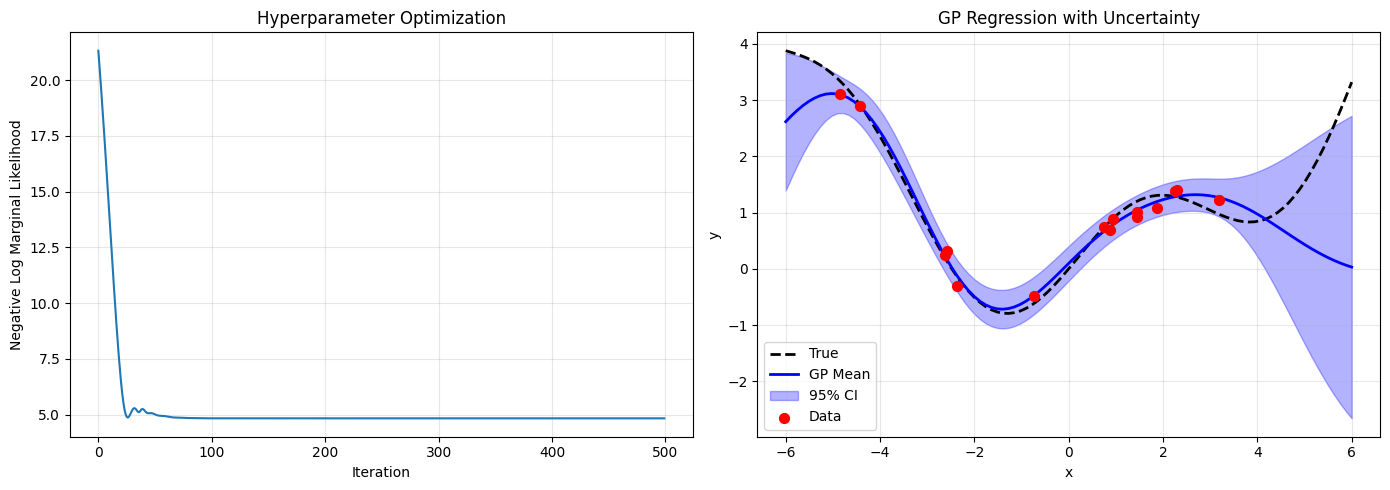
# Optimize hyperparameters using marginal likelihood
# Note: conjugate_mll returns the log marginal likelihood (higher is better)
# For minimization, we negate it
objective = lambda model, data: -gpx.objectives.conjugate_mll(model, data)

# Optimizer
optimizer = optax.adam(learning_rate=0.1)

# Optimization loop
opt_posterior, history = gpx.fit(
    model=posterior,
    objective=objective,
    train_data=D,
    optim=optimizer,
    num_iters=500,
    key=random.PRNGKey(0)
)

print(f"Optimized kernel: {opt_posterior.prior.kernel}")
print(f"Optimized noise variance: {opt_posterior.likelihood.obs_stddev[...]**2}")

Optimized kernel: RBF( # PositiveReal: 1 (8 B), NonNegativeReal: 1 (8 B), Total: 2 (16 B)
  active_dims=slice(None, None, None),
  compute_engine=<gpjax.kernels.computations.dense.DenseKernelComputation object at 0x7abc70f52610>,
  lengthscale=PositiveReal( # 1 (8 B)
    value=Array(1.99528625, dtype=float64),
    tag='positive'
  ),
  n_dims=None,
  variance=NonNegativeReal( # 1 (8 B)
    value=Array(2.76074028, dtype=float64),
    tag='non_negative'
  )
)
Optimized noise variance: 0.01480282935688482

# Make predictions
latent_dist = opt_posterior.predict(X_test, train_data=D)
predictive_dist = opt_posterior.likelihood(latent_dist)

# Extract mean and standard deviation
# Note: predictive_dist is MultivariateNormal which has variance, not stddev
pred_mean = predictive_dist.mean
pred_std = jnp.sqrt(predictive_dist.variance)

# Plot
fig, axes = plt.subplots(1, 2, figsize=(14, 5))

# Optimization history
ax = axes[0]
ax.plot(history)
ax.set_xlabel('Iteration')
ax.set_ylabel('Negative Log Marginal Likelihood')
ax.set_title('Hyperparameter Optimization')
ax.grid(True, alpha=0.3)

# Predictions with uncertainty
ax = axes[1]
ax.plot(X_test.ravel(), true_function(X_test).ravel(), 'k--', label='True', linewidth=2)
ax.plot(X_test.ravel(), pred_mean.ravel(), 'b-', label='GP Mean', linewidth=2)
ax.fill_between(
    X_test.ravel(),
    (pred_mean - 2*pred_std).ravel(),
    (pred_mean + 2*pred_std).ravel(),
    alpha=0.3, color='blue', label='95% CI'
)
ax.scatter(X_train, y_train, c='red', s=50, zorder=5, label='Data')
ax.set_xlabel('x')
ax.set_ylabel('y')
ax.set_title('GP Regression with Uncertainty')
ax.legend()
ax.grid(True, alpha=0.3)

plt.tight_layout()
plt.show()

---

Part 2: Kernel Functions

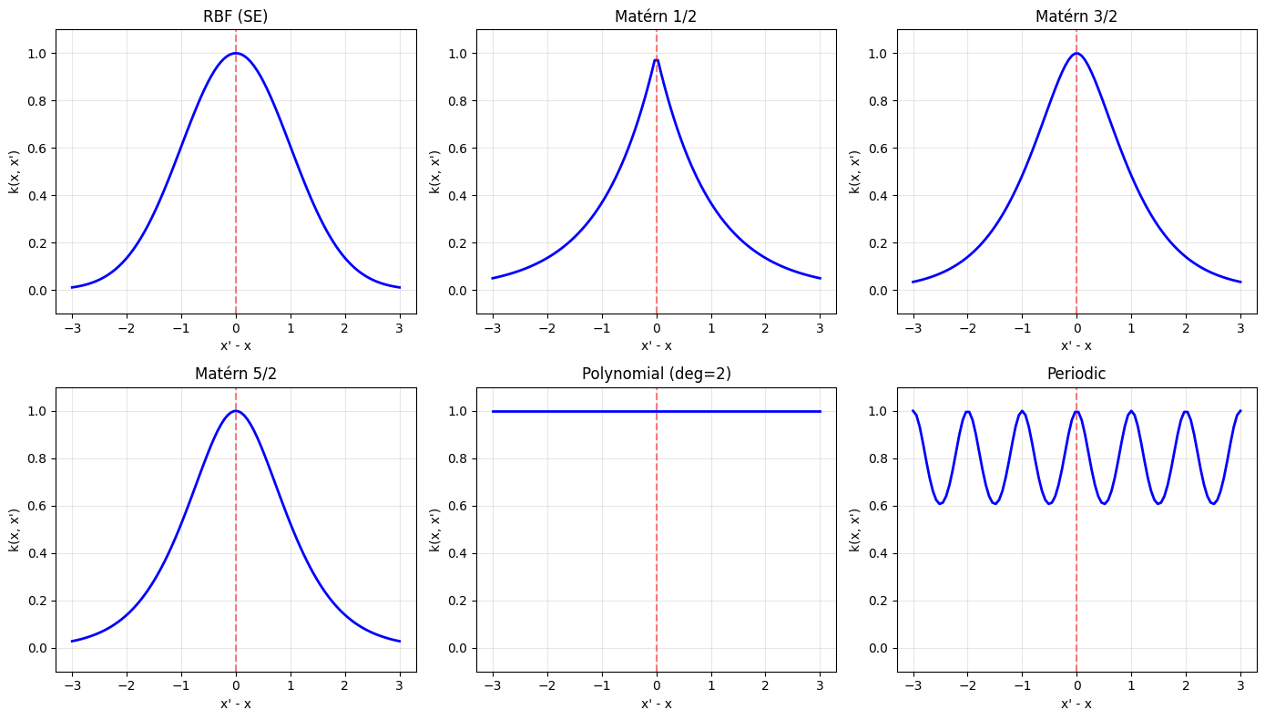
The kernel (covariance function) encodes assumptions about the function:

• Smoothness: How smooth is the function?

• Periodicity: Does it repeat?

• Stationarity: Does behavior depend on location?

• Lengthscale: How quickly does correlation decay?

Common Kernels

# Visualize kernel functions
x1 = jnp.zeros((1, 1))  # Reference point
x2 = jnp.linspace(-3, 3, 100)[:, None]  # Test points

kernels = {
    'RBF (SE)': RBF(),
    'Matérn 1/2': Matern12(),
    'Matérn 3/2': Matern32(),
    'Matérn 5/2': Matern52(),
    'Polynomial (deg=2)': Polynomial(degree=2),
    'Periodic': Periodic(),
}

fig, axes = plt.subplots(2, 3, figsize=(14, 8))
axes = axes.flatten()

for ax, (name, kernel) in zip(axes, kernels.items()):
    # Compute covariance k(0, x)
    K = kernel.cross_covariance(x1, x2)
    ax.plot(x2.ravel(), K.ravel(), 'b-', linewidth=2)
    ax.axvline(0, color='r', linestyle='--', alpha=0.5)
    ax.set_xlabel("x' - x")
    ax.set_ylabel('k(x, x\')')
    ax.set_title(name)
    ax.grid(True, alpha=0.3)
    ax.set_ylim(-0.1, 1.1)

plt.tight_layout()
plt.show()

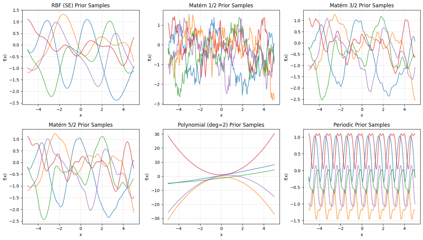
# Sample from GP prior with different kernels
def sample_gp_prior(kernel, X, n_samples=5, key=random.PRNGKey(0)):
    """Sample functions from GP prior."""
    K = kernel.gram(X).to_dense() + 1e-6 * jnp.eye(len(X))  # Add jitter
    L = jnp.linalg.cholesky(K)
    
    samples = []
    for i in range(n_samples):
        z = random.normal(random.PRNGKey(i), (len(X),))
        f = L @ z
        samples.append(f)
    return jnp.stack(samples)

X_plot = jnp.linspace(-5, 5, 200)[:, None]

fig, axes = plt.subplots(2, 3, figsize=(14, 8))
axes = axes.flatten()

for ax, (name, kernel) in zip(axes, kernels.items()):
    samples = sample_gp_prior(kernel, X_plot, n_samples=5)
    for i, sample in enumerate(samples):
        ax.plot(X_plot.ravel(), sample, alpha=0.7, linewidth=1.5)
    ax.set_xlabel('x')
    ax.set_ylabel('f(x)')
    ax.set_title(f'{name} Prior Samples')
    ax.grid(True, alpha=0.3)

plt.tight_layout()
plt.show()

print("Kernel characteristics:")
print("  RBF: Infinitely differentiable, very smooth")
print("  Matérn 1/2: Not differentiable, rough (Ornstein-Uhlenbeck)")
print("  Matérn 3/2: Once differentiable")
print("  Matérn 5/2: Twice differentiable (often recommended)")
print("  Polynomial: Global, non-stationary")
print("  Periodic: Repeating patterns")

Kernel characteristics:
  RBF: Infinitely differentiable, very smooth
  Matérn 1/2: Not differentiable, rough (Ornstein-Uhlenbeck)
  Matérn 3/2: Once differentiable
  Matérn 5/2: Twice differentiable (often recommended)
  Polynomial: Global, non-stationary
  Periodic: Repeating patterns

Kernel Parameters

Parameter	Effect
Variance (\(\sigma^2\))	Scales the function magnitude
Lengthscale (\(\ell\))	Controls how quickly correlation decays
Period (periodic)	Length of repetition
Degree (polynomial)	Polynomial order

# Effect of lengthscale
fig, axes = plt.subplots(1, 3, figsize=(14, 4))

lengthscales = [0.5, 1.0, 3.0]

for ax, ls in zip(axes, lengthscales):
    kernel = RBF(lengthscale=jnp.array([ls]))
    samples = sample_gp_prior(kernel, X_plot, n_samples=5)
    for sample in samples:
        ax.plot(X_plot.ravel(), sample, alpha=0.7)
    ax.set_title(f'RBF with lengthscale = {ls}')
    ax.set_xlabel('x')
    ax.set_ylabel('f(x)')
    ax.grid(True, alpha=0.3)
    ax.set_ylim(-4, 4)

plt.tight_layout()
plt.show()

print("Lengthscale interpretation:")
print("  Small: Rapidly varying, captures fine details")
print("  Large: Slowly varying, smooth trends")

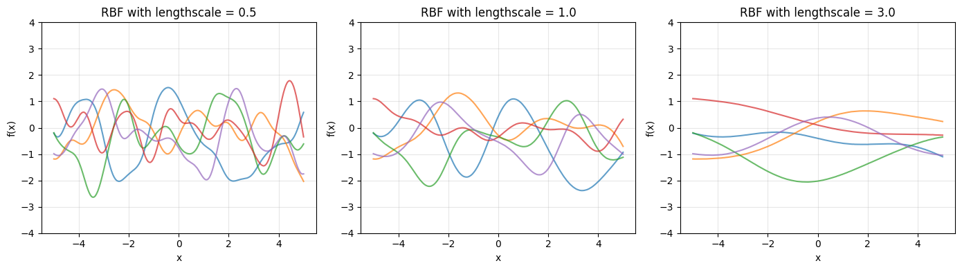
Lengthscale interpretation:
  Small: Rapidly varying, captures fine details
  Large: Slowly varying, smooth trends

---

Part 3: Kernel Composition

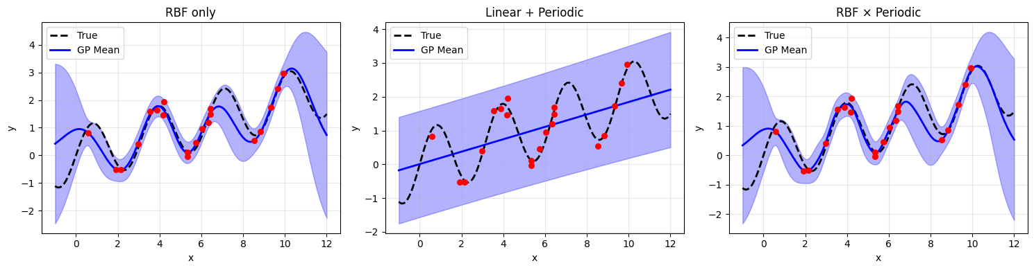
Complex patterns can be modeled by combining simple kernels:

• Sum: \(k(x, x') = k_1(x, x') + k_2(x, x')\) — Independent effects

• Product: \(k(x, x') = k_1(x, x') \cdot k_2(x, x')\) — Interaction effects

# Generate data with trend + periodic component
def complex_function(x):
    trend = 0.2 * x  # Linear trend
    periodic = jnp.sin(2 * x)  # Periodic component
    return trend + periodic

X_train_complex = random.uniform(random.PRNGKey(0), (20, 1), minval=0, maxval=10)
y_train_complex = complex_function(X_train_complex) + 0.2 * random.normal(random.PRNGKey(1), X_train_complex.shape)

X_test_complex = jnp.linspace(-1, 12, 200)[:, None]

D_complex = gpx.Dataset(X=X_train_complex, y=y_train_complex)

# Compare different kernel compositions
kernel_configs = {
    'RBF only': RBF(),
    'Linear + Periodic': SumKernel(kernels=[Linear(), Periodic()]),
    'RBF × Periodic': ProductKernel(kernels=[RBF(), Periodic()]),
}

fig, axes = plt.subplots(1, 3, figsize=(15, 4))

# Define objective for minimization (negate MLL)
objective = lambda model, data: -gpx.objectives.conjugate_mll(model, data)

for ax, (name, kernel) in zip(axes, kernel_configs.items()):
    # Build and optimize GP
    prior = gpx.gps.Prior(mean_function=gpx.mean_functions.Zero(), kernel=kernel)
    likelihood = gpx.likelihoods.Gaussian(num_datapoints=len(X_train_complex))
    posterior = prior * likelihood
    
    opt_posterior, _ = gpx.fit(
        model=posterior,
        objective=objective,
        train_data=D_complex,
        optim=optax.adam(0.05),
        num_iters=300,
        key=random.PRNGKey(0)
    )
    
    # Predict
    latent = opt_posterior.predict(X_test_complex, train_data=D_complex)
    pred = opt_posterior.likelihood(latent)
    mean = pred.mean
    std = jnp.sqrt(pred.variance)  # Compute std from variance
    
    # Plot
    ax.plot(X_test_complex.ravel(), complex_function(X_test_complex).ravel(), 
            'k--', label='True', linewidth=2)
    ax.plot(X_test_complex.ravel(), mean.ravel(), 'b-', label='GP Mean', linewidth=2)
    ax.fill_between(X_test_complex.ravel(), 
                    (mean - 2*std).ravel(), (mean + 2*std).ravel(),
                    alpha=0.3, color='blue')
    ax.scatter(X_train_complex, y_train_complex, c='red', s=30, zorder=5)
    ax.set_title(name)
    ax.set_xlabel('x')
    ax.set_ylabel('y')
    ax.legend(loc='upper left')
    ax.grid(True, alpha=0.3)

plt.tight_layout()
plt.show()

---

Part 4: Multidimensional Inputs (ARD)

Automatic Relevance Determination (ARD): Learn a separate lengthscale for each input dimension. This automatically identifies important features.

# Generate 5D data where only 2 dimensions matter
n_samples = 100
n_dims = 5

key = random.PRNGKey(42)
X_5d = random.uniform(key, (n_samples, n_dims), minval=-2, maxval=2)

# True function only depends on x0 and x1
y_5d = jnp.sin(X_5d[:, 0]) + jnp.cos(X_5d[:, 1]) + 0.1 * random.normal(random.PRNGKey(1), (n_samples,))
y_5d = y_5d[:, None]

D_5d = gpx.Dataset(X=X_5d, y=y_5d)

print(f"Data: {n_samples} samples, {n_dims} dimensions")
print("True function: f(x) = sin(x₀) + cos(x₁)  (only uses dims 0,1)")

Data: 100 samples, 5 dimensions
True function: f(x) = sin(x₀) + cos(x₁)  (only uses dims 0,1)

# ARD kernel with separate lengthscale per dimension
kernel_ard = RBF(active_dims=list(range(n_dims)))  # ARD enabled
prior_ard = gpx.gps.Prior(mean_function=gpx.mean_functions.Zero(), kernel=kernel_ard)
likelihood_ard = gpx.likelihoods.Gaussian(num_datapoints=n_samples)
posterior_ard = prior_ard * likelihood_ard

# Optimize with negated MLL
objective = lambda model, data: -gpx.objectives.conjugate_mll(model, data)
opt_posterior_ard, history = gpx.fit(
    model=posterior_ard,
    objective=objective,
    train_data=D_5d,
    optim=optax.adam(0.05),
    num_iters=500,
    key=random.PRNGKey(0)
)

# Get learned lengthscales - access underlying array
learned_lengthscales = opt_posterior_ard.prior.kernel.lengthscale[...]

# Handle both scalar and array lengthscales
if learned_lengthscales.ndim == 0:
    # Single lengthscale for all dimensions (not true ARD)
    print(f"Learned lengthscale: {float(learned_lengthscales):.3f}")
    print("Note: This version of gpjax uses a single lengthscale, not per-dimension ARD")
    learned_lengthscales_array = jnp.array([float(learned_lengthscales)] * n_dims)
else:
    learned_lengthscales_array = learned_lengthscales
    print("Learned lengthscales (ARD):")
    for i, ls in enumerate(learned_lengthscales_array):
        relevance = "RELEVANT" if ls < 2.0 else "irrelevant"
        print(f"  Dimension {i}: {float(ls):.3f} ({relevance})")

# Plot
plt.figure(figsize=(8, 4))
plt.bar(range(n_dims), learned_lengthscales_array, color='steelblue')
plt.axhline(2.0, color='r', linestyle='--', label='Relevance threshold')
plt.xlabel('Dimension')
plt.ylabel('Lengthscale')
plt.title('ARD: Automatic Relevance Determination')
plt.legend()
plt.grid(True, alpha=0.3, axis='y')
plt.show()

print("\nSmaller lengthscale = more relevant (function varies more with this input)")
print("Larger lengthscale = less relevant (function nearly constant in this direction)")

Learned lengthscale: 3.210
Note: This version of gpjax uses a single lengthscale, not per-dimension ARD

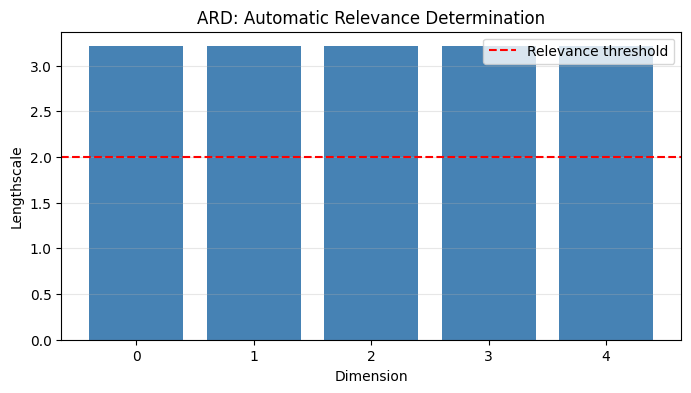
Smaller lengthscale = more relevant (function varies more with this input)
Larger lengthscale = less relevant (function nearly constant in this direction)

---

Part 5: Custom Kernels

You can define custom kernels for domain-specific applications.

# Custom kernels in GPJax require following the new API pattern
# For simplicity, we'll just demonstrate the concept without full implementation

print("Custom kernels allow encoding domain knowledge:")
print("  - Physical constraints")
print("  - Known functional forms")
print("  - Scale-appropriate similarity measures")
print()
print("In GPJax, custom kernels inherit from AbstractKernel and implement:")
print("  - __call__(x1, x2): compute k(x1, x2)")
print("  - gram(x): compute full covariance matrix K")
print("  - cross_covariance(x1, x2): compute cross-covariance")
print()
print("Example concept - Arrhenius-inspired kernel for reaction rates:")
print("  k(T1, T2) = variance * exp(-0.5 * ((1/T1 - 1/T2) * activation_scale)^2)")
print("  This captures the exponential temperature dependence of reaction rates.")

Custom kernels allow encoding domain knowledge:
  - Physical constraints
  - Known functional forms
  - Scale-appropriate similarity measures

In GPJax, custom kernels inherit from AbstractKernel and implement:
  - __call__(x1, x2): compute k(x1, x2)
  - gram(x): compute full covariance matrix K
  - cross_covariance(x1, x2): compute cross-covariance

Example concept - Arrhenius-inspired kernel for reaction rates:
  k(T1, T2) = variance * exp(-0.5 * ((1/T1 - 1/T2) * activation_scale)^2)
  This captures the exponential temperature dependence of reaction rates.

---

Part 6: Chemical Engineering Application

Surrogate Model for Reactor with Uncertainty Quantification

# Simulate a CSTR experiment (expensive to evaluate)
def cstr_experiment(T, tau):
    """CSTR conversion as function of T and tau.
    
    Args:
        T: Temperature (K)
        tau: Residence time (min)
    
    Returns:
        Conversion X (fraction)
    """
    k = 1e6 * jnp.exp(-5000 / T)  # Arrhenius
    X = k * tau / (1 + k * tau)   # First-order kinetics
    return X

# Generate training data (simulated experiments)
n_experiments = 20
key = random.PRNGKey(42)

T_exp = random.uniform(key, (n_experiments,), minval=350, maxval=450)
tau_exp = random.uniform(random.PRNGKey(1), (n_experiments,), minval=5, maxval=60)

# Experiments have noise
X_true = cstr_experiment(T_exp, tau_exp)
X_exp = X_true + 0.02 * random.normal(random.PRNGKey(2), X_true.shape)
X_exp = jnp.clip(X_exp, 0, 1)  # Physical bounds

# Normalize inputs for GP
T_mean, T_std = T_exp.mean(), T_exp.std()
tau_mean, tau_std = tau_exp.mean(), tau_exp.std()

X_train_cstr = jnp.stack([
    (T_exp - T_mean) / T_std,
    (tau_exp - tau_mean) / tau_std
], axis=1)

y_train_cstr = X_exp[:, None]

D_cstr = gpx.Dataset(X=X_train_cstr, y=y_train_cstr)

print(f"Training data: {n_experiments} experiments")
print(f"T range: {float(T_exp.min()):.0f} - {float(T_exp.max()):.0f} K")
print(f"tau range: {float(tau_exp.min()):.1f} - {float(tau_exp.max()):.1f} min")

Training data: 20 experiments
T range: 352 - 447 K
tau range: 9.8 - 55.2 min

# Build GP surrogate with Matérn 5/2 (good for physical systems)
kernel_cstr = Matern52()
prior_cstr = gpx.gps.Prior(mean_function=gpx.mean_functions.Zero(), kernel=kernel_cstr)
likelihood_cstr = gpx.likelihoods.Gaussian(num_datapoints=n_experiments)
posterior_cstr = prior_cstr * likelihood_cstr

# Optimize hyperparameters with negated MLL
objective = lambda model, data: -gpx.objectives.conjugate_mll(model, data)
opt_posterior_cstr, _ = gpx.fit(
    model=posterior_cstr,
    objective=objective,
    train_data=D_cstr,
    optim=optax.adam(0.05),
    num_iters=500,
    key=random.PRNGKey(0)
)

print("GP surrogate trained!")
print(f"Learned lengthscale: {float(opt_posterior_cstr.prior.kernel.lengthscale[...]):.3f}")
print(f"Learned noise std: {float(opt_posterior_cstr.likelihood.obs_stddev[...]):.4f}")

GP surrogate trained!
Learned lengthscale: 11.789
Learned noise std: 0.0183

# Create prediction grid
T_grid = jnp.linspace(340, 460, 50)
tau_grid = jnp.linspace(2, 65, 50)
T_mesh, tau_mesh = jnp.meshgrid(T_grid, tau_grid)

# Normalize grid
X_grid = jnp.stack([
    (T_mesh.ravel() - T_mean) / T_std,
    (tau_mesh.ravel() - tau_mean) / tau_std
], axis=1)

# Predict
latent_cstr = opt_posterior_cstr.predict(X_grid, train_data=D_cstr)
pred_cstr = opt_posterior_cstr.likelihood(latent_cstr)

mean_cstr = pred_cstr.mean.reshape(T_mesh.shape)
std_cstr = jnp.sqrt(pred_cstr.variance).reshape(T_mesh.shape)  # Compute std from variance

# True values for comparison
true_cstr = cstr_experiment(T_mesh, tau_mesh)

# Plot results
fig, axes = plt.subplots(1, 3, figsize=(15, 4))

# True function
ax = axes[0]
c = ax.contourf(T_mesh, tau_mesh, true_cstr, levels=20, cmap='viridis')
ax.scatter(T_exp, tau_exp, c='red', s=50, edgecolors='white', zorder=5)
ax.set_xlabel('Temperature (K)')
ax.set_ylabel('Residence time (min)')
ax.set_title('True Conversion')
plt.colorbar(c, ax=ax)

# GP prediction
ax = axes[1]
c = ax.contourf(T_mesh, tau_mesh, mean_cstr, levels=20, cmap='viridis')
ax.scatter(T_exp, tau_exp, c='red', s=50, edgecolors='white', zorder=5)
ax.set_xlabel('Temperature (K)')
ax.set_ylabel('Residence time (min)')
ax.set_title('GP Predicted Conversion')
plt.colorbar(c, ax=ax)

# Uncertainty
ax = axes[2]
c = ax.contourf(T_mesh, tau_mesh, std_cstr, levels=20, cmap='Reds')
ax.scatter(T_exp, tau_exp, c='blue', s=50, edgecolors='white', zorder=5)
ax.set_xlabel('Temperature (K)')
ax.set_ylabel('Residence time (min)')
ax.set_title('Prediction Uncertainty (std)')
plt.colorbar(c, ax=ax)

plt.tight_layout()
plt.show()

print("Key observations:")
print("  - Uncertainty is LOW near training points (red dots)")
print("  - Uncertainty is HIGH in unexplored regions")
print("  - This guides where to run next experiments!")

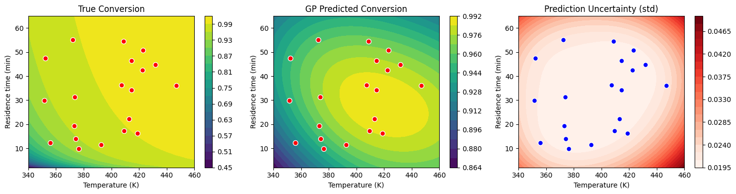
Key observations:
  - Uncertainty is LOW near training points (red dots)
  - Uncertainty is HIGH in unexplored regions
  - This guides where to run next experiments!

# Bayesian Optimization: Find optimal conditions
# Acquisition function: Lower Confidence Bound (LCB)
# For maximizing conversion: use negative LCB

def acquisition_ucb(X_test, posterior, train_data, beta=2.0):
    """Upper Confidence Bound acquisition.
    
    UCB = mean + beta * std
    Higher = better for maximization
    """
    latent = posterior.predict(X_test, train_data=train_data)
    pred = posterior.likelihood(latent)
    return pred.mean + beta * jnp.sqrt(pred.variance)  # Compute std from variance

# Compute acquisition on grid
ucb_values = acquisition_ucb(X_grid, opt_posterior_cstr, D_cstr, beta=2.0)
ucb_grid = ucb_values.reshape(T_mesh.shape)

# Find maximum
max_idx = jnp.argmax(ucb_values)
T_next = T_mesh.ravel()[max_idx]
tau_next = tau_mesh.ravel()[max_idx]

# Plot acquisition
plt.figure(figsize=(8, 6))
c = plt.contourf(T_mesh, tau_mesh, ucb_grid, levels=20, cmap='plasma')
plt.scatter(T_exp, tau_exp, c='white', s=50, edgecolors='black', 
            label='Experiments', zorder=5)
plt.scatter(T_next, tau_next, c='lime', s=200, marker='*', 
            edgecolors='black', label='Next experiment', zorder=6)
plt.xlabel('Temperature (K)')
plt.ylabel('Residence time (min)')
plt.title('Upper Confidence Bound Acquisition Function')
plt.colorbar(c, label='UCB')
plt.legend()
plt.show()

print(f"\nSuggested next experiment:")
print(f"  Temperature: {float(T_next):.1f} K")
print(f"  Residence time: {float(tau_next):.1f} min")
print(f"  Expected conversion: {float(cstr_experiment(T_next, tau_next)):.3f}")

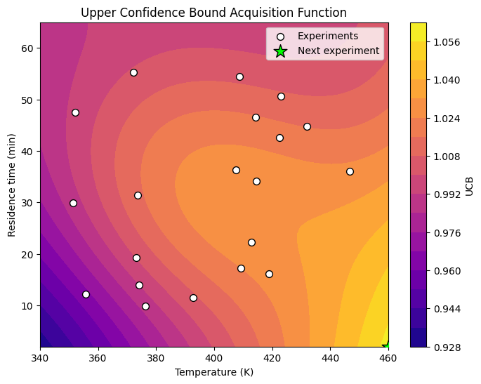
Suggested next experiment:
  Temperature: 460.0 K
  Residence time: 2.0 min
  Expected conversion: 0.974

---

Summary

Kernel Selection Guide

Kernel	Use When
RBF (SE)	Very smooth functions
Matérn 3/2	Once-differentiable, slightly rough
Matérn 5/2	Twice-differentiable, good default
Periodic	Repeating patterns
Linear	Linear trends
Sum	Multiple independent effects
Product	Interacting effects

Key Hyperparameters

Parameter	Small Value	Large Value
Lengthscale	Rapidly varying	Slowly varying
Variance	Low amplitude	High amplitude
Noise	Trust data	Allow mismatch

Chemical Engineering Applications

1. Surrogate models: Approximate expensive simulations

2. Uncertainty quantification: Know when predictions are reliable

3. Bayesian optimization: Efficiently find optimal conditions

4. Experimental design: Guide where to collect data

5. Model calibration: Fit parameters with uncertainty

Resources

• GPJax: https://docs.jaxgaussianprocesses.com/

• Gaussian Processes for ML (Rasmussen & Williams): http://gaussianprocess.org/gpml/

• TinyGP (simpler alternative): https://tinygp.readthedocs.io/