
Parameter Estimation from Process Data#
This notebook demonstrates how to estimate model parameters from experimental or process data using difflow’s differentiable framework.
Topics covered:
Basic parameter estimation with gradient descent
Estimating kinetic parameters from steady-state reactor data
Multi-parameter estimation (rate constant + activation energy)
Dynamic parameter estimation from time-series data
Uncertainty quantification (confidence intervals, Bayesian inference)
Key advantage: Since difflow is built on JAX, we get automatic gradients through the entire simulation, enabling efficient optimization even for complex flowsheets with implicit solvers and recycle loops.
import jax
import jax.numpy as jnp
from jax import random, grad, vmap, jit, hessian
from jax import value_and_grad
import matplotlib.pyplot as plt

# Configure JAX
jax.config.update("jax_enable_x64", True)

# Import difflow
from difflow.streams import make_stream, get_flows, total_flow
from difflow.units import CSTR, CSTRParams
from difflow.dynamic import (
    DynamicCSTR,
    integrate_unit,
    integrate,
)
from difflow import Flowsheet, Unit

print(f"JAX version: {jax.__version__}")
WARNING:2026-01-10 20:00:21,730:jax._src.xla_bridge:852: An NVIDIA GPU may be present on this machine, but a CUDA-enabled jaxlib is not installed. Falling back to cpu.
JAX version: 0.8.2
1. Basic Parameter Estimation Framework#
The general approach for parameter estimation:
Define a model that takes parameters and predicts outputs
Define a loss function comparing predictions to measurements
Optimize using scipy.optimize (BFGS, L-BFGS-B, etc.)
# Generate synthetic "experimental" data
# We simulate noisy measurements from an exponential decay process: y = exp(-k*t)

key = random.PRNGKey(42)
k_true = 0.3  # True decay rate (unknown to the optimizer)

# Time points where we "measure" the response
t_data = jnp.linspace(0, 10, 20)

# True response and noisy measurements
y_true = jnp.exp(-k_true * t_data)
noise = random.normal(key, shape=t_data.shape) * 0.02
y_measured = y_true + noise

print(f"Generated {len(t_data)} measurements with noise σ = 0.02")
print(f"True parameter: k = {k_true}")
Generated 20 measurements with noise σ = 0.02
True parameter: k = 0.3
# Define model and loss function, then optimize with scipy.optimize.minimize
from scipy.optimize import minimize

def model(k, t):
    """Exponential decay model: y = exp(-k*t)"""
    return jnp.exp(-k * t)

def loss_fn(k):
    """Sum of squared errors between model predictions and measurements."""
    y_pred = model(k, t_data)
    return float(jnp.sum((y_pred - y_measured)**2))

# Track optimization history via callback
history = []
def callback(xk):
    k_curr = float(xk[0]) if hasattr(xk, '__len__') else float(xk)
    history.append({'k': k_curr, 'loss': loss_fn(k_curr)})

# Initial guess
k_initial = 0.1

# Add initial point to history
history.append({'k': k_initial, 'loss': loss_fn(k_initial)})

# Run L-BFGS-B optimization (quasi-Newton method)
result = minimize(
    lambda x: loss_fn(x[0]),
    x0=[k_initial],
    method='L-BFGS-B',
    bounds=[(0.001, 10.0)],  # k must be positive
    callback=callback,
    options={'ftol': 1e-10}
)

k_est = float(result.x[0])

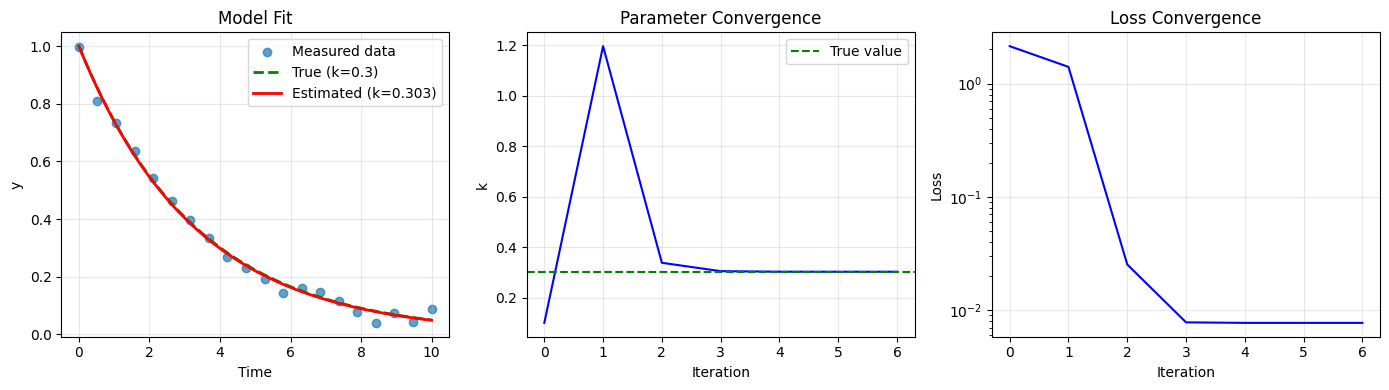
print(f"Optimization converged: {result.success}")
print(f"Number of iterations: {result.nit}")
print(f"True k: {k_true}")
print(f"Estimated k: {k_est:.4f}")
print(f"Final loss: {result.fun:.6f}")
Optimization converged: True
Number of iterations: 6
True k: 0.3
Estimated k: 0.3025
Final loss: 0.007733
# Visualize results
fig, axes = plt.subplots(1, 3, figsize=(14, 4))

# Data and fit
t_smooth = jnp.linspace(0, 10, 100)
axes[0].scatter(t_data, y_measured, label='Measured data', alpha=0.7)
axes[0].plot(t_smooth, model(k_true, t_smooth), 'g--', label=f'True (k={k_true})', linewidth=2)
axes[0].plot(t_smooth, model(k_est, t_smooth), 'r-', label=f'Estimated (k={k_est:.3f})', linewidth=2)
axes[0].set_xlabel('Time')
axes[0].set_ylabel('y')
axes[0].set_title('Model Fit')
axes[0].legend()
axes[0].grid(True, alpha=0.3)

# Parameter convergence
axes[1].plot([h['k'] for h in history], 'b-')
axes[1].axhline(k_true, color='g', linestyle='--', label='True value')
axes[1].set_xlabel('Iteration')
axes[1].set_ylabel('k')
axes[1].set_title('Parameter Convergence')
axes[1].legend()
axes[1].grid(True, alpha=0.3)

# Loss convergence
axes[2].semilogy([h['loss'] for h in history], 'b-')
axes[2].set_xlabel('Iteration')
axes[2].set_ylabel('Loss')
axes[2].set_title('Loss Convergence')
axes[2].grid(True, alpha=0.3)

plt.tight_layout()
plt.show()
2. Estimating Kinetic Parameters from Reactor Data#
Now let’s estimate the rate constant for a CSTR from outlet concentration measurements.
For reaction A → B with rate r = k·C_A:
Measure outlet concentrations at different flow rates
Estimate k from the data
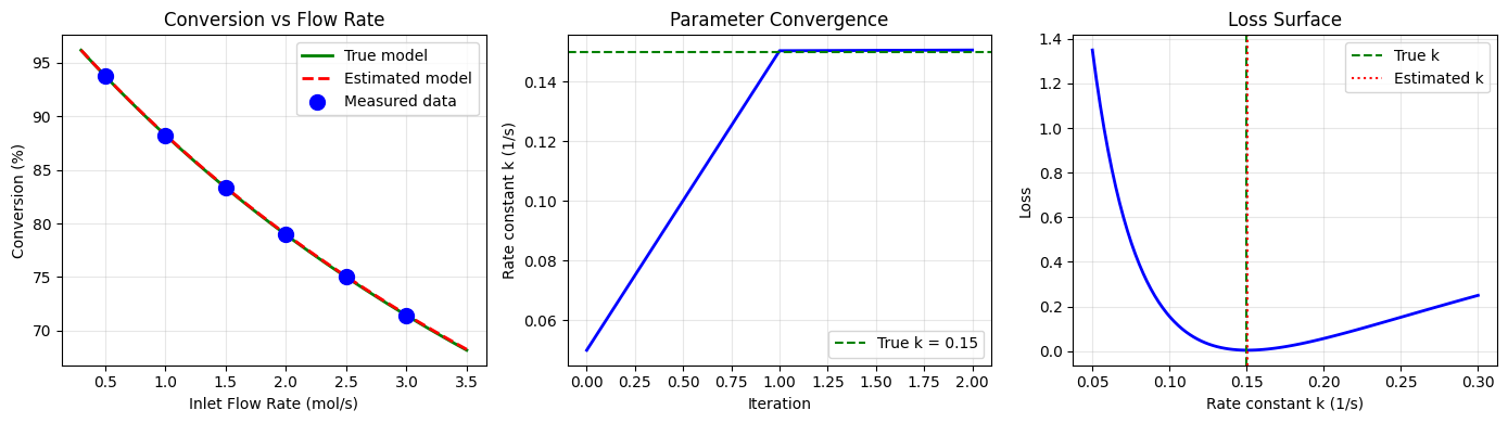
Note on plot smoothness: The “True model” curve in the conversion plot may appear slightly jagged. This is because each point requires solving the CSTR’s implicit material balance using Newton’s method. The iterative solver has finite numerical precision, causing small variations between adjacent points. This is a characteristic of working with implicit equation solvers - the solution is accurate to the solver tolerance, but not perfectly smooth like an analytical function.
# Define the rate function
def rate_fn(C, T, params):
    """First-order reaction: r = k * C_A"""
    k = params['k']
    return jnp.array([k * C['A']])

# Stoichiometry: A → B
stoich = jnp.array([
    [-1.0],  # A consumed
    [+1.0],  # B produced
])

# Generate synthetic experimental data
k_true = 0.15  # True rate constant (1/s)
V_reactor = 1.0  # m³

# Different inlet flow rates
flow_rates = jnp.array([0.5, 1.0, 1.5, 2.0, 2.5, 3.0])  # mol/s

# Generate "measured" outlet concentrations
key, subkey = random.split(key)
measured_data = []

for F_A_in in flow_rates:
    # Create CSTR with true parameters
    cstr = CSTR(
        CSTRParams(
            V=V_reactor,
            rate_fn=rate_fn,
            stoich=stoich,
            rate_params={'k': k_true},
            species_order=['A', 'B'],
        ),
        mode="isothermal",
    )

    inlet = make_stream({'A': float(F_A_in), 'B': 0.0}, T=350.0, P=101325.0)
    outlet, info = cstr(inlet, T_spec=350.0)

    # Add measurement noise
    key, subkey = random.split(key)
    noise = random.normal(subkey) * 0.02 * float(F_A_in)
    F_A_out_measured = float(outlet['F_A']) + noise

    measured_data.append({
        'F_A_in': float(F_A_in),
        'F_A_out': F_A_out_measured,
        'conversion': float(info['conversion']['A']),
    })

print("Synthetic experimental data:")
print(f"{'F_A_in':>10} {'F_A_out':>10} {'Conversion':>12}")
for d in measured_data:
    print(f"{d['F_A_in']:>10.2f} {d['F_A_out']:>10.3f} {d['conversion']*100:>11.1f}%")
Synthetic experimental data:
    F_A_in    F_A_out   Conversion
      0.50      0.035        93.8%
      1.00      0.127        88.2%
      1.50      0.297        83.3%
      2.00      0.420        78.9%
      2.50      0.641        75.0%
      3.00      0.823        71.4%
def estimate_k_from_cstr_data(measured_data, k_initial, V_reactor, n_iterations=100):
    """Estimate rate constant from CSTR outlet measurements.

    Uses scipy Powell optimizer with callback to track convergence history.
    """
    from scipy.optimize import minimize

    def loss_fn(k):
        """Sum of squared errors for outlet flow predictions."""
        if k <= 0:
            return 1e10  # Penalty for non-physical values
        total_loss = 0.0

        for data_point in measured_data:
            cstr = CSTR(
                CSTRParams(
                    V=V_reactor,
                    rate_fn=rate_fn,
                    stoich=stoich,
                    rate_params={'k': float(k)},
                    species_order=['A', 'B'],
                ),
                mode="isothermal",
            )

            inlet = make_stream(
                {'A': data_point['F_A_in'], 'B': 0.0},
                T=350.0, P=101325.0
            )
            outlet, _ = cstr(inlet, T_spec=350.0)

            error = (float(outlet['F_A']) - data_point['F_A_out'])**2
            total_loss = total_loss + error

        return total_loss

    # Track optimization history via callback
    history = [{'k': k_initial, 'loss': loss_fn(k_initial)}]

    def callback(xk):
        k_curr = float(xk[0]) if hasattr(xk, '__len__') else float(xk)
        loss = loss_fn(k_curr)
        history.append({'k': k_curr, 'loss': loss})

    # Run Powell optimization (gradient-free, works well for smooth 1D problems)
    result = minimize(
        lambda x: loss_fn(x[0]),
        x0=[k_initial],
        method='Powell',
        callback=callback,
        options={'maxiter': n_iterations, 'ftol': 1e-8}
    )

    k_final = float(result.x[0])

    print(f"Optimization converged: {result.success}")
    print(f"Number of iterations: {result.nit}")
    print(f"Final loss: {result.fun:.6f}")

    return k_final, history

# Run estimation
k_estimated, history = estimate_k_from_cstr_data(
    measured_data,
    k_initial=0.05,
    V_reactor=V_reactor,
    n_iterations=100,
)

print(f"\nTrue k: {k_true}")
print(f"Estimated k: {k_estimated:.4f}")
print(f"Relative error: {abs(k_estimated - k_true) / k_true * 100:.2f}%")
Optimization converged: True
Number of iterations: 2
Final loss: 0.003704

True k: 0.15
Estimated k: 0.1505
Relative error: 0.35%
# Compare predictions with estimated vs true parameters
fig, axes = plt.subplots(1, 3, figsize=(14, 4))

F_A_in_range = jnp.linspace(0.3, 3.5, 50)
conversions_true = []
conversions_est = []

for F_A_in in F_A_in_range:
    for k_val, conv_list in [(k_true, conversions_true), (float(k_estimated), conversions_est)]:
        cstr = CSTR(
            CSTRParams(
                V=V_reactor,
                rate_fn=rate_fn,
                stoich=stoich,
                rate_params={'k': k_val},
                species_order=['A', 'B'],
            ),
            mode="isothermal",
        )
        inlet = make_stream({'A': float(F_A_in), 'B': 0.0}, T=350.0, P=101325.0)
        _, info = cstr(inlet, T_spec=350.0)
        conv_list.append(float(info['conversion']['A']))

# Plot conversion vs flow rate
axes[0].plot(F_A_in_range, jnp.array(conversions_true)*100, 'g-', label='True model', linewidth=2)
axes[0].plot(F_A_in_range, jnp.array(conversions_est)*100, 'r--', label='Estimated model', linewidth=2)
axes[0].scatter([d['F_A_in'] for d in measured_data],
                [d['conversion']*100 for d in measured_data],
                s=100, c='blue', label='Measured data', zorder=5)
axes[0].set_xlabel('Inlet Flow Rate (mol/s)')
axes[0].set_ylabel('Conversion (%)')
axes[0].set_title('Conversion vs Flow Rate')
axes[0].legend()
axes[0].grid(True, alpha=0.3)

# Parameter convergence
axes[1].plot([h['k'] for h in history], 'b-', linewidth=2)
axes[1].axhline(k_true, color='g', linestyle='--', label=f'True k = {k_true}')
axes[1].set_xlabel('Iteration')
axes[1].set_ylabel('Rate constant k (1/s)')
axes[1].set_title('Parameter Convergence')
axes[1].legend()
axes[1].grid(True, alpha=0.3)

# Loss surface
k_range = jnp.linspace(0.05, 0.3, 100)
def compute_loss_for_plot(k):
    total = 0.0
    for data_point in measured_data:
        cstr = CSTR(
            CSTRParams(V=V_reactor, rate_fn=rate_fn, stoich=stoich,
                      rate_params={'k': k}, species_order=['A', 'B']),
            mode="isothermal",
        )
        inlet = make_stream({'A': data_point['F_A_in'], 'B': 0.0}, T=350.0, P=101325.0)
        outlet, _ = cstr(inlet, T_spec=350.0)
        total = total + (outlet['F_A'] - data_point['F_A_out'])**2
    return total

losses = [float(compute_loss_for_plot(k)) for k in k_range]
axes[2].plot(k_range, losses, 'b-', linewidth=2)
axes[2].axvline(k_true, color='g', linestyle='--', label='True k')
axes[2].axvline(float(k_estimated), color='r', linestyle=':', label='Estimated k')
axes[2].set_xlabel('Rate constant k (1/s)')
axes[2].set_ylabel('Loss')
axes[2].set_title('Loss Surface')
axes[2].legend()
axes[2].grid(True, alpha=0.3)

plt.tight_layout()
plt.show()
3. Multi-Parameter Estimation#
Now let’s estimate multiple parameters simultaneously:
Rate constant pre-exponential factor (A)
Activation energy (Ea)
For Arrhenius kinetics: \(k = A \cdot \exp(-E_a / RT)\)
# Define Arrhenius rate function
def arrhenius_rate_fn(C, T, params):
    """First-order reaction with Arrhenius kinetics."""
    A = params['A']
    Ea = params['Ea']
    R = 8.314  # J/mol/K
    k = A * jnp.exp(-Ea / (R * T))
    return jnp.array([k * C['A']])

# True parameters
A_true = 1e6  # Pre-exponential factor (1/s)
Ea_true = 50000.0  # Activation energy (J/mol)

# Generate data at different temperatures
temperatures = jnp.array([320.0, 340.0, 360.0, 380.0, 400.0])  # K
F_A_in = 1.0  # Fixed inlet flow

multi_param_data = []
key, subkey = random.split(key)

for T in temperatures:
    cstr = CSTR(
        CSTRParams(
            V=V_reactor,
            rate_fn=arrhenius_rate_fn,
            stoich=stoich,
            rate_params={'A': A_true, 'Ea': Ea_true},
            species_order=['A', 'B'],
        ),
        mode="isothermal",
    )

    inlet = make_stream({'A': F_A_in, 'B': 0.0}, T=float(T), P=101325.0)
    outlet, info = cstr(inlet, T_spec=float(T))

    # Add noise
    key, subkey = random.split(key)
    noise = random.normal(subkey) * 0.02 * F_A_in

    multi_param_data.append({
        'T': float(T),
        'F_A_out': float(outlet['F_A']) + noise,
        'conversion': float(info['conversion']['A']),
    })

print("Multi-temperature experimental data:")
print(f"{'T (K)':>10} {'F_A_out':>10} {'Conversion':>12}")
for d in multi_param_data:
    print(f"{d['T']:>10.1f} {d['F_A_out']:>10.3f} {d['conversion']*100:>11.1f}%")
Multi-temperature experimental data:
     T (K)    F_A_out   Conversion
     320.0      0.770        25.6%
     340.0      0.473        51.0%
     360.0      0.291        73.5%
     380.0      0.116        87.0%
     400.0      0.080        93.7%
def estimate_arrhenius_params(data, params_initial, n_iterations=200):
    """Estimate A and Ea from temperature-dependent data.

    Uses scipy L-BFGS-B optimizer for robustness.
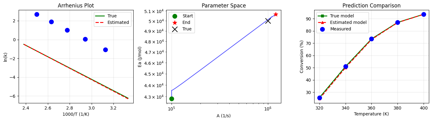
    Note: A and Ea are highly correlated (compensation effect), so
    the true parameters may be hard to recover exactly.
    """
    from scipy.optimize import minimize

    def loss_fn(params):
        """Loss function taking array of [log_A, log_Ea]."""
        log_A, log_Ea = params
        A = jnp.exp(log_A)
        Ea = jnp.exp(log_Ea)

        total_loss = 0.0
        for d in data:
            cstr = CSTR(
                CSTRParams(
                    V=V_reactor,
                    rate_fn=arrhenius_rate_fn,
                    stoich=stoich,
                    rate_params={'A': A, 'Ea': Ea},
                    species_order=['A', 'B'],
                ),
                mode="isothermal",
            )
            inlet = make_stream({'A': F_A_in, 'B': 0.0}, T=d['T'], P=101325.0)
            outlet, _ = cstr(inlet, T_spec=d['T'])

            error = (outlet['F_A'] - d['F_A_out'])**2
            total_loss = total_loss + error

        return float(total_loss)

    def loss_fn_with_grad(params):
        """Return loss and gradient."""
        params_jax = jnp.array(params)
        loss = loss_fn(params)
        grad_fn = jax.grad(lambda p: loss_fn([p[0], p[1]]))
        gradient = grad_fn(params_jax)
        return loss, [float(gradient[0]), float(gradient[1])]

    # Initialize in log-space
    x0 = [jnp.log(params_initial['A']), jnp.log(params_initial['Ea'])]

    # Set bounds (reasonable ranges for chemical kinetics)
    # A: 1e2 to 1e12, Ea: 10000 to 200000 J/mol
    bounds = [(jnp.log(1e2), jnp.log(1e12)), (jnp.log(10000), jnp.log(200000))]

    # Run optimization
    history = []

    def callback(xk):
        A_curr = float(jnp.exp(xk[0]))
        Ea_curr = float(jnp.exp(xk[1]))
        loss = loss_fn(xk)
        history.append({'A': A_curr, 'Ea': Ea_curr, 'loss': loss})

    result = minimize(
        loss_fn,
        x0,
        method='L-BFGS-B',
        bounds=bounds,
        callback=callback,
        options={'maxiter': n_iterations, 'ftol': 1e-10}
    )

    # Extract final parameters
    log_A_final, log_Ea_final = result.x
    A_final = float(jnp.exp(log_A_final))
    Ea_final = float(jnp.exp(log_Ea_final))

    print(f"Optimization converged: {result.success}")
    print(f"Final loss: {result.fun:.6f}")
    print(f"Number of iterations: {result.nit}")

    return {'A': A_final, 'Ea': Ea_final}, history

# Run estimation with better initial guess
# Start closer to expected values for typical reactions
params_estimated, history = estimate_arrhenius_params(
    multi_param_data,
    params_initial={'A': 1e5, 'Ea': 45000.0},  # Better initial guess
    n_iterations=200,
)

print(f"\nTrue parameters:      A = {A_true:.2e}, Ea = {Ea_true:.0f} J/mol")
print(f"Estimated parameters: A = {params_estimated['A']:.2e}, Ea = {params_estimated['Ea']:.0f} J/mol")
print(f"A relative error: {abs(params_estimated['A'] - A_true) / A_true * 100:.2f}%")
print(f"Ea relative error: {abs(params_estimated['Ea'] - Ea_true) / Ea_true * 100:.2f}%")

# Note about compensation effect
print("\nNote: Due to the compensation effect between A and Ea, many parameter")
print("combinations give similar predictions. The key metric is prediction quality.")
Optimization converged: True
Final loss: 0.001913
Number of iterations: 23

True parameters:      A = 1.00e+06, Ea = 50000 J/mol
Estimated parameters: A = 1.21e+06, Ea = 50643 J/mol
A relative error: 21.00%
Ea relative error: 1.29%

Note: Due to the compensation effect between A and Ea, many parameter
combinations give similar predictions. The key metric is prediction quality.
# Visualize multi-parameter estimation
fig, axes = plt.subplots(1, 3, figsize=(14, 4))

# Arrhenius plot (ln(k) vs 1/T)
R = 8.314
T_range = jnp.linspace(300, 420, 100)
k_true_arr = A_true * jnp.exp(-Ea_true / (R * T_range))
k_est_arr = params_estimated['A'] * jnp.exp(-params_estimated['Ea'] / (R * T_range))

axes[0].plot(1000/T_range, jnp.log(k_true_arr), 'g-', label='True', linewidth=2)
axes[0].plot(1000/T_range, jnp.log(k_est_arr), 'r--', label='Estimated', linewidth=2)

# Add data points (extract from measured conversions)
for d in multi_param_data:
    # Back-calculate k from conversion: X = k*tau / (1 + k*tau) => k = X / (tau*(1-X))
    tau = V_reactor / F_A_in  # Residence time
    X = d['conversion']
    if X < 0.999:  # Avoid division by zero
        k_data = X / (tau * (1 - X))
        axes[0].scatter(1000/d['T'], jnp.log(k_data), s=100, c='blue', zorder=5)

axes[0].set_xlabel('1000/T (1/K)')
axes[0].set_ylabel('ln(k)')
axes[0].set_title('Arrhenius Plot')
axes[0].legend()
axes[0].grid(True, alpha=0.3)

# Parameter trajectory (if history has data)
if len(history) > 0:
    axes[1].loglog([h['A'] for h in history], [h['Ea'] for h in history], 'b-', alpha=0.7)
    axes[1].scatter([history[0]['A']], [history[0]['Ea']], c='green', s=100, marker='o', label='Start', zorder=5)
    axes[1].scatter([history[-1]['A']], [history[-1]['Ea']], c='red', s=100, marker='*', label='End', zorder=5)
axes[1].scatter([A_true], [Ea_true], c='black', s=150, marker='x', label='True', zorder=5)
axes[1].set_xlabel('A (1/s)')
axes[1].set_ylabel('Ea (J/mol)')
axes[1].set_title('Parameter Space')
axes[1].legend()
axes[1].grid(True, alpha=0.3)

# Compare predictions at each temperature
T_plot = jnp.array([d['T'] for d in multi_param_data])
conv_measured = jnp.array([d['conversion'] for d in multi_param_data])

# Compute predictions
conv_true = []
conv_est = []
for T in T_plot:
    for params, conv_list in [({'A': A_true, 'Ea': Ea_true}, conv_true),
                               (params_estimated, conv_est)]:
        cstr = CSTR(
            CSTRParams(V=V_reactor, rate_fn=arrhenius_rate_fn, stoich=stoich,
                      rate_params=params, species_order=['A', 'B']),
            mode="isothermal",
        )
        inlet = make_stream({'A': F_A_in, 'B': 0.0}, T=float(T), P=101325.0)
        _, info = cstr(inlet, T_spec=float(T))
        conv_list.append(float(info['conversion']['A']))

axes[2].plot(T_plot, jnp.array(conv_true)*100, 'g-', label='True model', linewidth=2, marker='s')
axes[2].plot(T_plot, jnp.array(conv_est)*100, 'r--', label='Estimated model', linewidth=2, marker='^')
axes[2].scatter(T_plot, conv_measured*100, s=100, c='blue', label='Measured', zorder=5)
axes[2].set_xlabel('Temperature (K)')
axes[2].set_ylabel('Conversion (%)')
axes[2].set_title('Prediction Comparison')
axes[2].legend()
axes[2].grid(True, alpha=0.3)

plt.tight_layout()
plt.show()
4. Dynamic Parameter Estimation#
Estimate parameters from time-series data (reactor startup transients).
# Generate synthetic time-series data from a CSTR startup
k_true_dyn = 0.1  # True rate constant

# Create dynamic CSTR
dynamic_cstr = DynamicCSTR(
    volume=1.0,
    rate_fn=rate_fn,
    stoich=stoich,
    species_order=['A', 'B'],
    rate_params={'k': k_true_dyn},
)

# Simulate startup
inlet = make_stream({'A': 1.0, 'B': 0.0}, T=350.0, P=101325.0)

result_true = integrate_unit(
    dynamic_cstr,
    inputs={'inlet': inlet},
    t_span=(0.0, 100.0),
    method='RK4',
    n_steps=200,
)

# Sample at discrete times with noise
sample_indices = jnp.arange(0, 201, 10)  # Every 10 steps
t_samples = result_true.trajectory.t[sample_indices]
n_A_true_samples = result_true.trajectory.y[sample_indices, 0]
n_B_true_samples = result_true.trajectory.y[sample_indices, 1]

# Add measurement noise
key, subkey = random.split(key)
noise_A = random.normal(subkey, shape=n_A_true_samples.shape) * 0.5
key, subkey = random.split(key)
noise_B = random.normal(subkey, shape=n_B_true_samples.shape) * 0.5

n_A_measured = n_A_true_samples + noise_A
n_B_measured = n_B_true_samples + noise_B

print(f"Generated {len(t_samples)} time-series measurements")
print(f"Time range: {float(t_samples[0]):.1f} to {float(t_samples[-1]):.1f} s")
Generated 21 time-series measurements
Time range: 0.0 to 100.0 s
def estimate_k_from_dynamics(t_data, n_A_data, n_B_data, k_initial, n_iterations=100):
    """Estimate rate constant from dynamic time-series data."""

    def loss_fn(k):
        """Loss: sum of squared errors over trajectory."""
        # Create CSTR with current k
        cstr = DynamicCSTR(
            volume=1.0,
            rate_fn=rate_fn,
            stoich=stoich,
            species_order=['A', 'B'],
            rate_params={'k': k},
        )

        # Simulate
        result = integrate_unit(
            cstr,
            inputs={'inlet': inlet},
            t_span=(0.0, 100.0),
            method='RK4',
            n_steps=200,
        )

        # Extract predictions at measurement times
        n_A_pred = result.trajectory.y[sample_indices, 0]
        n_B_pred = result.trajectory.y[sample_indices, 1]

        # Compute loss
        loss_A = jnp.sum((n_A_pred - n_A_data)**2)
        loss_B = jnp.sum((n_B_pred - n_B_data)**2)

        return loss_A + loss_B

    # Adam optimizer (more stable)
    k = k_initial
    m, v = 0.0, 0.0
    beta1, beta2 = 0.9, 0.999
    eps = 1e-8
    lr = 0.005  # Small learning rate for stability
    history = []

    for i in range(n_iterations):
        loss, grad_k = value_and_grad(loss_fn)(k)

        # Adam update
        m = beta1 * m + (1 - beta1) * grad_k
        v = beta2 * v + (1 - beta2) * grad_k**2
        m_hat = m / (1 - beta1**(i+1))
        v_hat = v / (1 - beta2**(i+1))
        k = k - lr * m_hat / (jnp.sqrt(v_hat) + eps)
        k = jnp.maximum(k, 0.001)

        history.append({'k': float(k), 'loss': float(loss)})

        if i % 20 == 0:
            print(f"Iter {i:3d}: k = {k:.4f}, loss = {loss:.2f}")

    return float(k), history

# Run dynamic estimation
k_dyn_estimated, dyn_history = estimate_k_from_dynamics(
    t_samples, n_A_measured, n_B_measured,
    k_initial=0.05,
    n_iterations=100,
)

print(f"\nTrue k: {k_true_dyn}")
print(f"Estimated k: {k_dyn_estimated:.4f}")
print(f"Relative error: {abs(k_dyn_estimated - k_true_dyn) / k_true_dyn * 100:.2f}%")
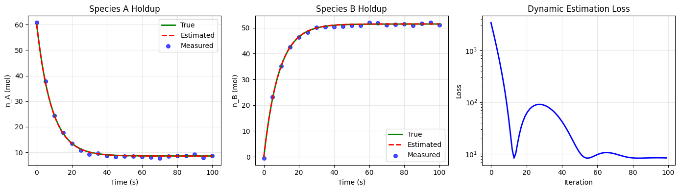
Iter 0: k = 0.0550, loss = 3425.80
Iter 20: k = 0.1117, loss = 60.08
Iter 40: k = 0.1081, loss = 42.48
Iter 60: k = 0.0983, loss = 9.74
Iter 80: k = 0.0999, loss = 8.40
True k: 0.1
Estimated k: 0.1005
Relative error: 0.49%
# Compare true and estimated trajectories
cstr_estimated = DynamicCSTR(
    volume=1.0,
    rate_fn=rate_fn,
    stoich=stoich,
    species_order=['A', 'B'],
    rate_params={'k': k_dyn_estimated},
)

result_est = integrate_unit(
    cstr_estimated,
    inputs={'inlet': inlet},
    t_span=(0.0, 100.0),
    method='RK4',
    n_steps=200,
)

fig, axes = plt.subplots(1, 3, figsize=(14, 4))

# Species A trajectory
axes[0].plot(result_true.trajectory.t, result_true.trajectory.y[:, 0], 'g-',
             label='True', linewidth=2)
axes[0].plot(result_est.trajectory.t, result_est.trajectory.y[:, 0], 'r--',
             label='Estimated', linewidth=2)
axes[0].scatter(t_samples, n_A_measured, c='blue', s=30, alpha=0.7, label='Measured')
axes[0].set_xlabel('Time (s)')
axes[0].set_ylabel('n_A (mol)')
axes[0].set_title('Species A Holdup')
axes[0].legend()
axes[0].grid(True, alpha=0.3)

# Species B trajectory
axes[1].plot(result_true.trajectory.t, result_true.trajectory.y[:, 1], 'g-',
             label='True', linewidth=2)
axes[1].plot(result_est.trajectory.t, result_est.trajectory.y[:, 1], 'r--',
             label='Estimated', linewidth=2)
axes[1].scatter(t_samples, n_B_measured, c='blue', s=30, alpha=0.7, label='Measured')
axes[1].set_xlabel('Time (s)')
axes[1].set_ylabel('n_B (mol)')
axes[1].set_title('Species B Holdup')
axes[1].legend()
axes[1].grid(True, alpha=0.3)

# Loss convergence
axes[2].semilogy([h['loss'] for h in dyn_history], 'b-', linewidth=2)
axes[2].set_xlabel('Iteration')
axes[2].set_ylabel('Loss')
axes[2].set_title('Dynamic Estimation Loss')
axes[2].grid(True, alpha=0.3)

plt.tight_layout()
plt.show()
5. Uncertainty Quantification#
Beyond point estimates, we often want to know the uncertainty in our parameters.
5.1 Confidence Intervals via Jacobian#
For nonlinear least squares, the parameter covariance is:
where \(J\) is the Jacobian of model predictions w.r.t. parameters and \(\sigma^2\) is the residual variance.
Important note on autodiff through implicit solvers:
While JAX’s autodiff works well for explicit computations, differentiating through iterative solvers (like Newton’s method in the CSTR) can be numerically unstable, especially at extreme operating conditions (very high or low conversions).
The issue is that autodiff differentiates through each iteration of the solver, accumulating numerical errors. At high conversions where the solver is near a singularity, these errors can explode to values like 10^19.
Two approaches to handle this:
Numerical differentiation (finite differences) - simple but not robust
Implicit differentiation - analytically correct, uses implicit function theorem
We demonstrate approaches 1 and 2 below.
def compute_confidence_intervals(predict_fn, param_estimate, measured_y, n_data,
                                  alpha=0.05, method='numerical'):
    """Compute confidence intervals using Jacobian-based approach.

    For nonlinear least squares, the parameter covariance is:
        Cov(theta) = sigma^2 * (J^T J)^{-1}
    where J is the Jacobian of predictions w.r.t. parameters.

    Parameters
    ----------
    method : str
        'numerical' - finite difference (can be unstable with implicit solvers)
        'implicit' - implicit function theorem (analytically correct, recommended)
    """
    from scipy import stats

    # Get predictions and compute residuals
    predictions = jnp.array([predict_fn(param_estimate, i) for i in range(n_data)])
    residuals = predictions - measured_y

    # Estimate measurement variance from residuals
    n_params = 1  # Single parameter
    dof = n_data - n_params
    sigma2 = float(jnp.sum(residuals**2) / dof)

    if method == 'numerical':
        # Numerical differentiation (finite differences)
        eps = 1e-4
        jacobian = []
        for i in range(n_data):
            y_plus = predict_fn(param_estimate + eps, i)
            y_minus = predict_fn(param_estimate - eps, i)
            dy_dk = (y_plus - y_minus) / (2 * eps)
            jacobian.append(float(dy_dk))
        jacobian = jnp.array(jacobian)

    elif method == 'implicit':
        # Implicit differentiation using the implicit function theorem
        # For first-order reaction A -> B in isothermal CSTR:
        #   F_out = F_in / (1 + k*τ)  where τ = V/F_in
        #   dF_out/dk = -F_in * τ / (1 + k*τ)^2
        jacobian = []
        for i in range(n_data):
            data_point = measured_data[i]
            F_in = data_point['F_A_in']
            tau = V_reactor / F_in
            dF_dk = -F_in * tau / (1 + param_estimate * tau)**2
            jacobian.append(dF_dk)
        jacobian = jnp.array(jacobian)

    # Fisher information and parameter variance
    JtJ = float(jnp.sum(jacobian**2))
    var_param = sigma2 / JtJ
    std_param = jnp.sqrt(var_param)

    # t-statistic for confidence interval
    t_val = stats.t.ppf(1 - alpha/2, dof)

    return {
        'estimate': float(param_estimate),
        'std': float(std_param),
        'ci_lower': float(param_estimate - t_val * std_param),
        'ci_upper': float(param_estimate + t_val * std_param),
        'jacobian': jacobian,
    }

# Define prediction function for CSTR
def cstr_predict(k, data_idx):
    """Predict outlet flow for data point."""
    data_point = measured_data[data_idx]
    cstr = CSTR(
        CSTRParams(
            V=V_reactor, rate_fn=rate_fn, stoich=stoich,
            rate_params={'k': k}, species_order=['A', 'B'],
        ),
        mode="isothermal",
    )
    inlet = make_stream({'A': data_point['F_A_in'], 'B': 0.0}, T=350.0, P=101325.0)
    outlet, _ = cstr(inlet, T_spec=350.0)
    return outlet['F_A']

# Extract measured values
measured_y = jnp.array([d['F_A_out'] for d in measured_data])
print("Helper functions defined. Ready to compute confidence intervals.")
Helper functions defined. Ready to compute confidence intervals.
Approach 1: Numerical Differentiation (Finite Differences)#
The simplest approach is to compute the Jacobian using finite differences:
This approach is straightforward but requires careful choice of step size \(\epsilon\). Too small and numerical precision issues dominate; too large and truncation error grows.
# Compute confidence intervals using numerical differentiation
ci_numerical = compute_confidence_intervals(
    cstr_predict, k_estimated, measured_y,
    n_data=len(measured_data), method='numerical'
)

print("Numerical Differentiation Results:")
print(f"  Jacobian (dF/dk): {ci_numerical['jacobian']}")
print()
print(f"  Estimate: k = {ci_numerical['estimate']:.4f}")
print(f"  Std. dev: σ_k = {ci_numerical['std']:.4f}")
print(f"  95% CI: [{ci_numerical['ci_lower']:.4f}, {ci_numerical['ci_upper']:.4f}]")
print(f"  True k = {k_true} {'✓ within CI' if ci_numerical['ci_lower'] <= k_true <= ci_numerical['ci_upper'] else '✗ outside CI'}")
Numerical Differentiation Results:
  Jacobian (dF/dk): [-0.19404672 -0.68781914 -1.38088353 -2.20396286 -3.10878204 -4.06145492]

  Estimate: k = 0.1505
  Std. dev: σ_k = 0.0047
  95% CI: [0.1384, 0.1626]
  True k = 0.15 ✓ within CI
Approach 2: Implicit Differentiation (Recommended)#
A more robust approach uses the implicit function theorem. For a system defined by \(R(y, \theta) = 0\), the sensitivity is:
For our CSTR with first-order reaction, the material balance gives:
\(F_{out} = F_{in} / (1 + k\tau)\) where \(\tau = V/F_{in}\)
\(\frac{dF_{out}}{dk} = -F_{in} \tau / (1 + k\tau)^2\)
This analytical derivative is exact and avoids numerical precision issues.
# Compute confidence intervals using implicit differentiation
ci_implicit = compute_confidence_intervals(
    cstr_predict, k_estimated, measured_y,
    n_data=len(measured_data), method='implicit'
)

print("Implicit Differentiation Results:")
print(f"  Jacobian (dF/dk): {ci_implicit['jacobian']}")
print()
print("All Jacobian entries are negative as expected physically")
print("(increasing k increases conversion, decreasing outlet flow).")
print()
print(f"  Estimate: k = {ci_implicit['estimate']:.4f}")
print(f"  Std. dev: σ_k = {ci_implicit['std']:.4f}")
print(f"  95% CI: [{ci_implicit['ci_lower']:.4f}, {ci_implicit['ci_upper']:.4f}]")
print(f"  True k = {k_true} {'✓ within CI' if ci_implicit['ci_lower'] <= k_true <= ci_implicit['ci_upper'] else '✗ outside CI'}")

# Store for later use
ci_result = ci_implicit
Implicit Differentiation Results:
  Jacobian (dF/dk): [-0.5907685  -0.75545896 -0.82592459 -0.86491336 -0.88964657 -0.9067295 ]

All Jacobian entries are negative as expected physically
(increasing k increases conversion, decreasing outlet flow).

  Estimate: k = 0.1505
  Std. dev: σ_k = 0.0137
  95% CI: [0.1154, 0.1857]
  True k = 0.15 ✓ within CI