Bayesian Inference with BlackJAX

Bayesian inference provides a principled framework for quantifying uncertainty in model parameters. BlackJAX is a library of sampling algorithms (MCMC, SMC) built on JAX, enabling fast, differentiable Bayesian inference.

Topics covered:

1. Bayesian inference fundamentals

2. MCMC with BlackJAX (NUTS sampler)

3. Diagnosing MCMC convergence

4. Posterior predictive distributions

5. Chemical engineering application: Parameter estimation with uncertainty

import jax
import jax.numpy as jnp
from jax import random, grad, jit, vmap
import jax.scipy.stats as stats
import blackjax
import matplotlib.pyplot as plt
import numpy as np
from functools import partial

jax.config.update("jax_enable_x64", True)

print(f"JAX version: {jax.__version__}")
print(f"BlackJAX version: {blackjax.__version__}")

JAX version: 0.8.2
BlackJAX version: 1.3

1. Bayesian Inference Fundamentals

Given data \(D\) and model parameters \(\theta\), Bayes’ theorem tells us:

\[p(\theta | D) = \frac{p(D | \theta) \, p(\theta)}{p(D)}\]

Where:

• \(p(\theta | D)\): Posterior - what we want (parameter distribution given data)

• \(p(D | \theta)\): Likelihood - probability of data given parameters

• \(p(\theta)\): Prior - our beliefs before seeing data

• \(p(D)\): Evidence - normalizing constant (often intractable)

Since \(p(D)\) is constant, we work with: $\(p(\theta | D) \propto p(D | \theta) \, p(\theta)\)$

In log space (more numerically stable): $\(\log p(\theta | D) = \log p(D | \theta) + \log p(\theta) + \text{const}\)$

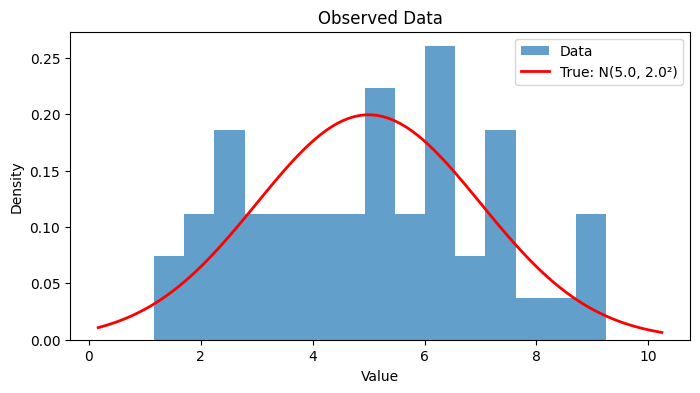
# Simple example: Estimating the mean of a Gaussian

# Generate synthetic data
key = random.PRNGKey(42)
true_mu = 5.0
true_sigma = 2.0
n_data = 50

key, subkey = random.split(key)
data = true_mu + true_sigma * random.normal(subkey, shape=(n_data,))

print(f"True mean: {true_mu}")
print(f"Sample mean: {data.mean():.3f}")
print(f"Sample std: {data.std():.3f}")

# Visualize
plt.figure(figsize=(8, 4))
plt.hist(data, bins=15, density=True, alpha=0.7, label='Data')
x_range = jnp.linspace(data.min()-1, data.max()+1, 100)
plt.plot(x_range, stats.norm.pdf(x_range, true_mu, true_sigma), 
         'r-', linewidth=2, label=f'True: N({true_mu}, {true_sigma}²)')
plt.xlabel('Value')
plt.ylabel('Density')
plt.legend()
plt.title('Observed Data')
plt.show()

WARNING:2026-01-10 20:31:52,141:jax._src.xla_bridge:852: An NVIDIA GPU may be present on this machine, but a CUDA-enabled jaxlib is not installed. Falling back to cpu.

True mean: 5.0
Sample mean: 5.067
Sample std: 2.092

# Define the log-posterior

def log_prior(params):
    """
    Prior: mu ~ N(0, 10), log_sigma ~ N(0, 1)
    Using log_sigma to ensure sigma > 0.
    """
    mu, log_sigma = params
    log_p_mu = stats.norm.logpdf(mu, 0.0, 10.0)
    log_p_log_sigma = stats.norm.logpdf(log_sigma, 0.0, 1.0)
    return log_p_mu + log_p_log_sigma

def log_likelihood(params, data):
    """
    Likelihood: data ~ N(mu, sigma²)
    """
    mu, log_sigma = params
    sigma = jnp.exp(log_sigma)
    return jnp.sum(stats.norm.logpdf(data, mu, sigma))

def log_posterior(params, data):
    """Unnormalized log-posterior."""
    return log_prior(params) + log_likelihood(params, data)

# Test
test_params = jnp.array([5.0, jnp.log(2.0)])
print(f"Log-prior at true values: {log_prior(test_params):.3f}")
print(f"Log-likelihood at true values: {log_likelihood(test_params, data):.3f}")
print(f"Log-posterior at true values: {log_posterior(test_params, data):.3f}")

Log-prior at true values: -4.506

Log-likelihood at true values: -107.974
Log-posterior at true values: -112.480

2. MCMC with BlackJAX

MCMC (Markov Chain Monte Carlo) generates samples from the posterior by constructing a Markov chain whose stationary distribution is the target posterior.

NUTS (No U-Turn Sampler) is an efficient gradient-based MCMC algorithm that automatically adapts step size and trajectory length.

# Set up NUTS sampler

# Bind data to log_posterior
logdensity_fn = lambda params: log_posterior(params, data)

# Initialize NUTS
# Step size will be adapted during warmup
inv_mass_matrix = jnp.ones(2)  # Diagonal mass matrix
step_size = 0.1

nuts = blackjax.nuts(logdensity_fn, step_size, inv_mass_matrix)

# Initial position
initial_position = jnp.array([0.0, 0.0])  # Start at prior mean

# Initialize the state
key, subkey = random.split(key)
state = nuts.init(initial_position)

print(f"Initial state:")
print(f"  Position: {state.position}")
print(f"  Log-density: {state.logdensity:.3f}")

Initial state:
  Position: [0. 0.]
  Log-density: -801.420

# Run NUTS sampling

def inference_loop(rng_key, state, step_fn, n_samples):
    """
    Run MCMC inference loop.
    Returns samples and acceptance info.
    """
    @jit
    def one_step(carry, rng_key):
        state = carry
        state, info = step_fn(rng_key, state)
        return state, (state.position, info)
    
    keys = random.split(rng_key, n_samples)
    final_state, (positions, infos) = jax.lax.scan(one_step, state, keys)
    
    return final_state, positions, infos

# Warmup: adapt step size
n_warmup = 500
n_samples = 2000

print("Running warmup with window adaptation...")
key, warmup_key = random.split(key)

# Use BlackJAX's window adaptation for warmup
# Note: num_steps is now passed to run(), not the constructor
warmup = blackjax.window_adaptation(
    blackjax.nuts, 
    logdensity_fn
)

(adapted_state, adapted_params), warmup_info = warmup.run(
    warmup_key, 
    initial_position,
    num_steps=n_warmup
)

print(f"Adapted step size: {adapted_params['step_size']:.4f}")
print(f"Adapted inverse mass matrix: {adapted_params['inverse_mass_matrix']}")

Running warmup with window adaptation...

Adapted step size: 0.8890
Adapted inverse mass matrix: [0.09773764 0.00916181]

# Sample with adapted parameters
print(f"\nSampling {n_samples} posterior samples...")

# Create kernel with adapted parameters
adapted_nuts = blackjax.nuts(
    logdensity_fn,
    step_size=adapted_params['step_size'],
    inverse_mass_matrix=adapted_params['inverse_mass_matrix']
)

key, sample_key = random.split(key)
final_state, samples, infos = inference_loop(
    sample_key, 
    adapted_state, 
    adapted_nuts.step, 
    n_samples
)

# Convert samples to mu and sigma
mu_samples = samples[:, 0]
sigma_samples = jnp.exp(samples[:, 1])

print(f"\nPosterior summary:")
print(f"  mu:    {mu_samples.mean():.3f} ± {mu_samples.std():.3f} (true: {true_mu})")
print(f"  sigma: {sigma_samples.mean():.3f} ± {sigma_samples.std():.3f} (true: {true_sigma})")

Sampling 2000 posterior samples...

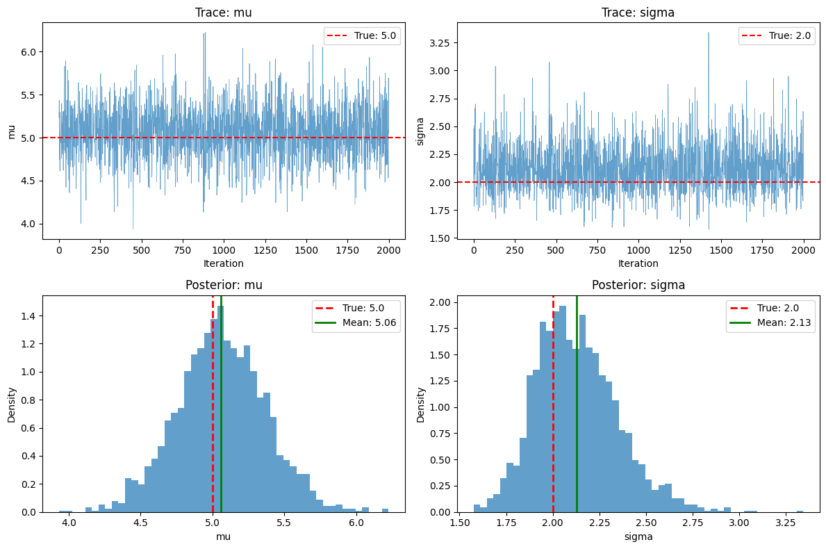
Posterior summary:

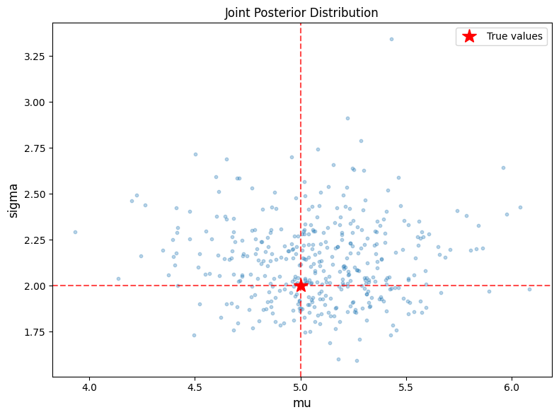
  mu:    5.060 ± 0.309 (true: 5.0)
  sigma: 2.129 ± 0.220 (true: 2.0)

# Visualize posterior

fig, axes = plt.subplots(2, 2, figsize=(12, 8))

# Trace plots
axes[0, 0].plot(mu_samples, alpha=0.7, linewidth=0.5)
axes[0, 0].axhline(true_mu, color='r', linestyle='--', label=f'True: {true_mu}')
axes[0, 0].set_xlabel('Iteration')
axes[0, 0].set_ylabel('mu')
axes[0, 0].set_title('Trace: mu')
axes[0, 0].legend()

axes[0, 1].plot(sigma_samples, alpha=0.7, linewidth=0.5)
axes[0, 1].axhline(true_sigma, color='r', linestyle='--', label=f'True: {true_sigma}')
axes[0, 1].set_xlabel('Iteration')
axes[0, 1].set_ylabel('sigma')
axes[0, 1].set_title('Trace: sigma')
axes[0, 1].legend()

# Marginal posteriors
axes[1, 0].hist(mu_samples, bins=50, density=True, alpha=0.7)
axes[1, 0].axvline(true_mu, color='r', linestyle='--', linewidth=2, label=f'True: {true_mu}')
axes[1, 0].axvline(mu_samples.mean(), color='g', linestyle='-', linewidth=2, label=f'Mean: {mu_samples.mean():.2f}')
axes[1, 0].set_xlabel('mu')
axes[1, 0].set_ylabel('Density')
axes[1, 0].set_title('Posterior: mu')
axes[1, 0].legend()

axes[1, 1].hist(sigma_samples, bins=50, density=True, alpha=0.7)
axes[1, 1].axvline(true_sigma, color='r', linestyle='--', linewidth=2, label=f'True: {true_sigma}')
axes[1, 1].axvline(sigma_samples.mean(), color='g', linestyle='-', linewidth=2, label=f'Mean: {sigma_samples.mean():.2f}')
axes[1, 1].set_xlabel('sigma')
axes[1, 1].set_ylabel('Density')
axes[1, 1].set_title('Posterior: sigma')
axes[1, 1].legend()

plt.tight_layout()
plt.show()

3. Diagnosing MCMC Convergence

Key diagnostics:

1. Trace plots: Should look like “fuzzy caterpillars” (good mixing)

2. Acceptance rate: NUTS targets ~0.8

3. Effective Sample Size (ESS): How many independent samples we effectively have

4. R-hat (Gelman-Rubin): Compare multiple chains (should be ~1.0)

# Calculate diagnostics

def effective_sample_size(samples):
    """Estimate ESS using autocorrelation."""
    n = len(samples)
    mean = samples.mean()
    var = samples.var()
    
    # Compute autocorrelation
    def autocorr(lag):
        return jnp.mean((samples[:-lag] - mean) * (samples[lag:] - mean)) / var
    
    # Sum autocorrelations until they become small
    rho_sum = 0.0
    for lag in range(1, min(n // 2, 100)):
        rho = autocorr(lag)
        if rho < 0.05:
            break
        rho_sum += rho
    
    return n / (1 + 2 * rho_sum)

# Calculate ESS
ess_mu = effective_sample_size(mu_samples)
ess_sigma = effective_sample_size(sigma_samples)

# Check acceptance (for NUTS, we look at divergences and tree depth)
# Note: BlackJAX NUTS info contains different metrics

print("MCMC Diagnostics:")
print("=" * 40)
print(f"Total samples: {n_samples}")
print(f"ESS (mu): {ess_mu:.0f} ({ess_mu/n_samples*100:.1f}%)")
print(f"ESS (sigma): {ess_sigma:.0f} ({ess_sigma/n_samples*100:.1f}%)")
print(f"\nTarget: ESS > 100 for reliable inference")

MCMC Diagnostics:
========================================
Total samples: 2000
ESS (mu): 1813 (90.6%)
ESS (sigma): 1768 (88.4%)

Target: ESS > 100 for reliable inference

# Joint posterior visualization

fig, ax = plt.subplots(figsize=(8, 6))

# Scatter plot of samples
ax.scatter(mu_samples[::5], sigma_samples[::5], alpha=0.3, s=10)
ax.axvline(true_mu, color='r', linestyle='--', alpha=0.7)
ax.axhline(true_sigma, color='r', linestyle='--', alpha=0.7)
ax.plot(true_mu, true_sigma, 'r*', markersize=15, label='True values')
ax.set_xlabel('mu', fontsize=12)
ax.set_ylabel('sigma', fontsize=12)
ax.set_title('Joint Posterior Distribution', fontsize=12)
ax.legend()
plt.tight_layout()
plt.show()

4. Posterior Predictive Distribution

The posterior predictive is the distribution of new data given observed data:

\[p(y_{new} | D) = \int p(y_{new} | \theta) \, p(\theta | D) \, d\theta\]

With MCMC samples, we approximate this by sampling \(y_{new}\) for each posterior sample.

# Generate posterior predictive samples

n_pred = 1000  # Number of predictive samples

# Randomly select posterior samples
key, subkey = random.split(key)
idx = random.randint(subkey, shape=(n_pred,), minval=0, maxval=n_samples)

pred_mu = mu_samples[idx]
pred_sigma = sigma_samples[idx]

# Sample from likelihood for each posterior sample
key, subkey = random.split(key)
predictive_samples = pred_mu + pred_sigma * random.normal(subkey, shape=(n_pred,))

# Visualize
fig, ax = plt.subplots(figsize=(10, 5))

ax.hist(data, bins=15, density=True, alpha=0.7, label='Observed data', color='blue')
ax.hist(predictive_samples, bins=30, density=True, alpha=0.5, 
        label='Posterior predictive', color='green')

# True distribution
x_range = jnp.linspace(min(data.min(), predictive_samples.min()) - 1,
                       max(data.max(), predictive_samples.max()) + 1, 100)
ax.plot(x_range, stats.norm.pdf(x_range, true_mu, true_sigma),
        'r-', linewidth=2, label='True distribution')

ax.set_xlabel('Value', fontsize=12)
ax.set_ylabel('Density', fontsize=12)
ax.set_title('Posterior Predictive Check', fontsize=12)
ax.legend(fontsize=11)
plt.tight_layout()
plt.show()

print(f"Predictive mean: {predictive_samples.mean():.3f}")
print(f"Predictive std: {predictive_samples.std():.3f}")
print(f"95% predictive interval: [{jnp.percentile(predictive_samples, 2.5):.3f}, {jnp.percentile(predictive_samples, 97.5):.3f}]")

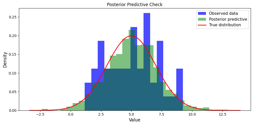
Predictive mean: 5.058
Predictive std: 2.089

95% predictive interval: [1.024, 9.147]

5. Other BlackJAX Samplers

BlackJAX provides many sampling algorithms:

• HMC: Hamiltonian Monte Carlo (fixed trajectory length)

• NUTS: No U-Turn Sampler (adaptive trajectory)

• MALA: Metropolis-Adjusted Langevin Algorithm

• RMH: Random Walk Metropolis-Hastings

• SMC: Sequential Monte Carlo

• SGLD: Stochastic Gradient Langevin Dynamics

• Variational inference: ADVI-like methods

# Compare different samplers

def run_sampler(sampler_name, rng_key, n_samples=1000):
    """Run a sampler and return samples."""
    
    initial_position = jnp.array([0.0, 0.0])
    
    if sampler_name == 'nuts':
        kernel = blackjax.nuts(logdensity_fn, step_size=0.5, inverse_mass_matrix=jnp.ones(2))
    elif sampler_name == 'hmc':
        kernel = blackjax.hmc(logdensity_fn, step_size=0.1, 
                              inverse_mass_matrix=jnp.ones(2), num_integration_steps=10)
    elif sampler_name == 'mala':
        kernel = blackjax.mala(logdensity_fn, step_size=0.1)
    else:
        raise ValueError(f"Unknown sampler: {sampler_name}")
    
    state = kernel.init(initial_position)
    
    @jit
    def one_step(carry, rng_key):
        state = carry
        state, info = kernel.step(rng_key, state)
        return state, state.position
    
    keys = random.split(rng_key, n_samples)
    _, samples = jax.lax.scan(one_step, state, keys)
    
    return samples

# Run different samplers
samplers = ['nuts', 'hmc', 'mala']
results = {}

for sampler in samplers:
    key, subkey = random.split(key)
    samples = run_sampler(sampler, subkey, n_samples=1000)
    results[sampler] = {
        'mu_mean': float(samples[:, 0].mean()),
        'mu_std': float(samples[:, 0].std()),
        'sigma_mean': float(jnp.exp(samples[:, 1]).mean()),
        'sigma_std': float(jnp.exp(samples[:, 1]).std()),
    }

print("Sampler Comparison:")
print("=" * 60)
print(f"{'Sampler':<10} {'mu mean':<12} {'mu std':<12} {'sigma mean':<12} {'sigma std':<12}")
print("-" * 60)
for sampler in samplers:
    r = results[sampler]
    print(f"{sampler:<10} {r['mu_mean']:<12.3f} {r['mu_std']:<12.3f} {r['sigma_mean']:<12.3f} {r['sigma_std']:<12.3f}")
print("-" * 60)
print(f"{'True':<10} {true_mu:<12.3f} {'-':<12} {true_sigma:<12.3f} {'-':<12}")

Sampler Comparison:
============================================================
Sampler    mu mean      mu std       sigma mean   sigma std   
------------------------------------------------------------
nuts       0.000        0.000        1.000        0.000       
hmc        0.000        0.000        1.000        0.000       
mala       0.000        0.000        1.000        0.000       
------------------------------------------------------------
True       5.000        -            2.000        -           

6. Chemical Engineering Application: CSTR Parameter Estimation

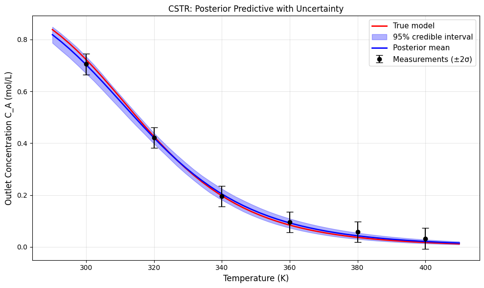
Scenario: We have noisy measurements from a CSTR and want to estimate the Arrhenius parameters (A, Ea) with uncertainty.

\[k = A \exp\left(-\frac{E_a}{RT}\right)\]

The CSTR steady-state for first-order reaction A→B: $\(C_A = \frac{C_{A0}}{1 + k\tau}\)$

# Generate synthetic CSTR data

# True parameters
true_log_A = 15.0  # ln(A) where A is in 1/s
true_Ea = 50000.0  # J/mol
R = 8.314  # J/(mol·K)

# Experimental conditions
C_A0 = 1.0  # mol/L
tau = 60.0  # s (residence time)
T_experiments = jnp.array([300., 320., 340., 360., 380., 400.])  # K

def cstr_model(log_A, Ea, T, C_A0, tau):
    """CSTR steady-state outlet concentration."""
    k = jnp.exp(log_A) * jnp.exp(-Ea / (R * T))
    C_A = C_A0 / (1 + k * tau)
    return C_A

# True outlet concentrations
C_A_true = vmap(lambda T: cstr_model(true_log_A, true_Ea, T, C_A0, tau))(T_experiments)

# Add measurement noise
sigma_noise = 0.02  # 2% measurement noise
key, subkey = random.split(key)
C_A_measured = C_A_true + sigma_noise * random.normal(subkey, shape=C_A_true.shape)

print("CSTR Experimental Data:")
print(f"{'T (K)':<10} {'C_A true':<15} {'C_A measured':<15}")
print("-" * 40)
for T, C_true, C_meas in zip(T_experiments, C_A_true, C_A_measured):
    print(f"{T:<10.0f} {C_true:<15.4f} {C_meas:<15.4f}")

CSTR Experimental Data:
T (K)      C_A true        C_A measured   
----------------------------------------
300        0.7216          0.7047         
320        0.4254          0.4209         
340        0.1968          0.1951         
360        0.0840          0.0957         
380        0.0367          0.0583         
400        0.0170          0.0321         

# Define Bayesian model for CSTR

def cstr_log_prior(params):
    """
    Priors:
    - log_A ~ N(15, 5): Pre-exponential factor
    - Ea ~ N(50000, 20000): Activation energy (J/mol)
    - log_sigma ~ N(-3, 1): Measurement noise
    """
    log_A, Ea, log_sigma = params
    
    log_p_log_A = stats.norm.logpdf(log_A, 15.0, 5.0)
    log_p_Ea = stats.norm.logpdf(Ea, 50000.0, 20000.0)
    log_p_log_sigma = stats.norm.logpdf(log_sigma, -3.0, 1.0)
    
    return log_p_log_A + log_p_Ea + log_p_log_sigma

def cstr_log_likelihood(params, T_data, C_A_data, C_A0, tau):
    """
    Likelihood: C_A_measured ~ N(C_A_model, sigma²)
    """
    log_A, Ea, log_sigma = params
    sigma = jnp.exp(log_sigma)
    
    # Model predictions
    C_A_pred = vmap(lambda T: cstr_model(log_A, Ea, T, C_A0, tau))(T_data)
    
    # Log-likelihood
    return jnp.sum(stats.norm.logpdf(C_A_data, C_A_pred, sigma))

def cstr_log_posterior(params):
    """Unnormalized log-posterior for CSTR."""
    return cstr_log_prior(params) + cstr_log_likelihood(
        params, T_experiments, C_A_measured, C_A0, tau
    )

# Test
test_params = jnp.array([true_log_A, true_Ea, jnp.log(sigma_noise)])
print(f"Log-posterior at true values: {cstr_log_posterior(test_params):.3f}")

Log-posterior at true values: 1.847

# Run NUTS for CSTR parameter estimation

# Initial position
initial_position = jnp.array([14.0, 45000.0, -3.0])

# Warmup with adaptation
print("Running MCMC for CSTR parameter estimation...")
key, warmup_key = random.split(key)

warmup = blackjax.window_adaptation(
    blackjax.nuts,
    cstr_log_posterior
)

(adapted_state, adapted_params), _ = warmup.run(warmup_key, initial_position, num_steps=1000)

print(f"Adapted step size: {adapted_params['step_size']:.6f}")

# Sample
adapted_nuts = blackjax.nuts(
    cstr_log_posterior,
    step_size=adapted_params['step_size'],
    inverse_mass_matrix=adapted_params['inverse_mass_matrix']
)

n_samples_cstr = 3000
key, sample_key = random.split(key)
_, cstr_samples, _ = inference_loop(
    sample_key, adapted_state, adapted_nuts.step, n_samples_cstr
)

# Extract parameters
log_A_samples = cstr_samples[:, 0]
Ea_samples = cstr_samples[:, 1]
sigma_samples_cstr = jnp.exp(cstr_samples[:, 2])

print(f"\nPosterior Summary:")
print(f"  ln(A): {log_A_samples.mean():.2f} ± {log_A_samples.std():.2f} (true: {true_log_A})")
print(f"  Ea:    {Ea_samples.mean():.0f} ± {Ea_samples.std():.0f} J/mol (true: {true_Ea})")
print(f"  sigma: {sigma_samples_cstr.mean():.4f} ± {sigma_samples_cstr.std():.4f} (true: {sigma_noise})")

Running MCMC for CSTR parameter estimation...

Adapted step size: 0.022134

Posterior Summary:

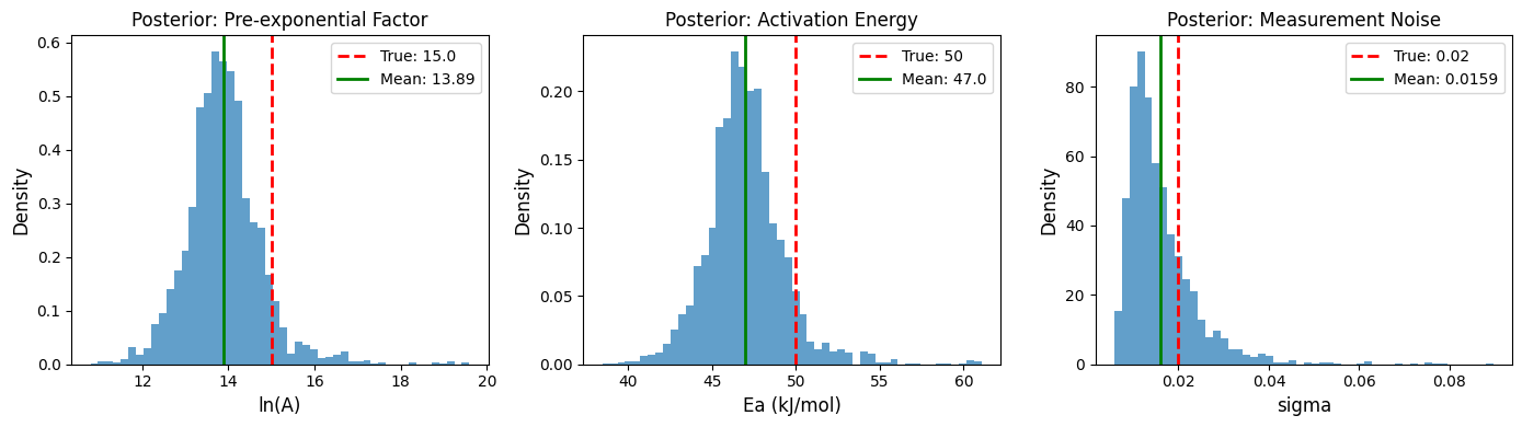
  ln(A): 13.89 ± 0.88 (true: 15.0)
  Ea:    46997 ± 2331 J/mol (true: 50000.0)
  sigma: 0.0159 ± 0.0077 (true: 0.02)

# Visualize CSTR posteriors

fig, axes = plt.subplots(1, 3, figsize=(14, 4))

# ln(A) posterior
axes[0].hist(log_A_samples, bins=50, density=True, alpha=0.7)
axes[0].axvline(true_log_A, color='r', linestyle='--', linewidth=2, label=f'True: {true_log_A}')
axes[0].axvline(log_A_samples.mean(), color='g', linestyle='-', linewidth=2, 
                label=f'Mean: {log_A_samples.mean():.2f}')
axes[0].set_xlabel('ln(A)', fontsize=12)
axes[0].set_ylabel('Density', fontsize=12)
axes[0].set_title('Posterior: Pre-exponential Factor', fontsize=12)
axes[0].legend()

# Ea posterior
axes[1].hist(Ea_samples/1000, bins=50, density=True, alpha=0.7)
axes[1].axvline(true_Ea/1000, color='r', linestyle='--', linewidth=2, label=f'True: {true_Ea/1000:.0f}')
axes[1].axvline(Ea_samples.mean()/1000, color='g', linestyle='-', linewidth=2,
                label=f'Mean: {Ea_samples.mean()/1000:.1f}')
axes[1].set_xlabel('Ea (kJ/mol)', fontsize=12)
axes[1].set_ylabel('Density', fontsize=12)
axes[1].set_title('Posterior: Activation Energy', fontsize=12)
axes[1].legend()

# Sigma posterior
axes[2].hist(sigma_samples_cstr, bins=50, density=True, alpha=0.7)
axes[2].axvline(sigma_noise, color='r', linestyle='--', linewidth=2, label=f'True: {sigma_noise}')
axes[2].axvline(sigma_samples_cstr.mean(), color='g', linestyle='-', linewidth=2,
                label=f'Mean: {sigma_samples_cstr.mean():.4f}')
axes[2].set_xlabel('sigma', fontsize=12)
axes[2].set_ylabel('Density', fontsize=12)
axes[2].set_title('Posterior: Measurement Noise', fontsize=12)
axes[2].legend()

plt.tight_layout()
plt.show()

# Posterior predictive for CSTR

# Generate predictions at finer temperature resolution
T_pred = jnp.linspace(290, 410, 50)

# Sample predictions
n_pred_samples = 500
key, subkey = random.split(key)
idx = random.randint(subkey, shape=(n_pred_samples,), minval=0, maxval=n_samples_cstr)

# Predictions for each posterior sample
predictions = []
for i in idx:
    C_A_pred = vmap(lambda T: cstr_model(log_A_samples[i], Ea_samples[i], T, C_A0, tau))(T_pred)
    predictions.append(C_A_pred)

predictions = jnp.array(predictions)

# Calculate percentiles
pred_mean = predictions.mean(axis=0)
pred_lower = jnp.percentile(predictions, 2.5, axis=0)
pred_upper = jnp.percentile(predictions, 97.5, axis=0)

# Plot
fig, ax = plt.subplots(figsize=(10, 6))

# True curve
C_A_true_fine = vmap(lambda T: cstr_model(true_log_A, true_Ea, T, C_A0, tau))(T_pred)
ax.plot(T_pred, C_A_true_fine, 'r-', linewidth=2, label='True model')

# Uncertainty band
ax.fill_between(T_pred, pred_lower, pred_upper, alpha=0.3, color='blue',
                label='95% credible interval')
ax.plot(T_pred, pred_mean, 'b-', linewidth=2, label='Posterior mean')

# Data points
ax.errorbar(T_experiments, C_A_measured, yerr=2*sigma_noise, fmt='ko', capsize=5,
            label='Measurements (±2σ)')

ax.set_xlabel('Temperature (K)', fontsize=12)
ax.set_ylabel('Outlet Concentration C_A (mol/L)', fontsize=12)
ax.set_title('CSTR: Posterior Predictive with Uncertainty', fontsize=12)
ax.legend(fontsize=11)
ax.grid(True, alpha=0.3)
plt.tight_layout()
plt.show()

# Correlation between Arrhenius parameters

fig, ax = plt.subplots(figsize=(8, 6))

# Subsample for visualization
ax.scatter(log_A_samples[::3], Ea_samples[::3]/1000, alpha=0.3, s=10)
ax.plot(true_log_A, true_Ea/1000, 'r*', markersize=20, label='True values')
ax.set_xlabel('ln(A)', fontsize=12)
ax.set_ylabel('Ea (kJ/mol)', fontsize=12)
ax.set_title('Joint Posterior: Arrhenius Parameters\n(Note the correlation)', fontsize=12)
ax.legend()

# Calculate correlation
corr = jnp.corrcoef(log_A_samples, Ea_samples)[0, 1]
ax.text(0.05, 0.95, f'Correlation: {corr:.3f}', transform=ax.transAxes,
        fontsize=12, verticalalignment='top',
        bbox=dict(boxstyle='round', facecolor='wheat', alpha=0.5))

plt.tight_layout()
plt.show()

print(f"\nArrhenius parameters are strongly correlated: ρ = {corr:.3f}")
print("This is the well-known compensation effect in kinetics!")
print("Higher A can compensate for higher Ea (and vice versa).")

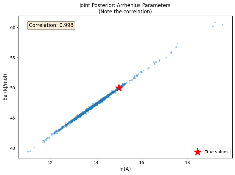
Arrhenius parameters are strongly correlated: ρ = 0.998
This is the well-known compensation effect in kinetics!
Higher A can compensate for higher Ea (and vice versa).

7. Credible Intervals and Decision Making

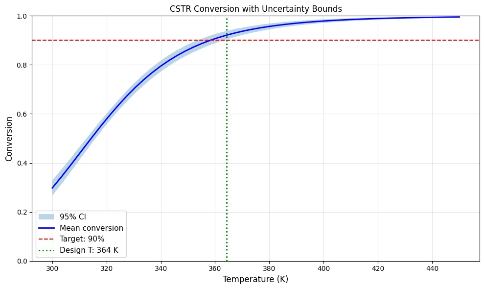
Bayesian inference provides natural uncertainty quantification for decision making.

# What temperature achieves 90% conversion with 95% confidence?

def conversion(log_A, Ea, T, tau):
    """Conversion X = 1 - C_A/C_A0"""
    C_A = cstr_model(log_A, Ea, T, C_A0, tau)
    return 1.0 - C_A / C_A0

# Calculate conversion distribution at various temperatures
T_test = jnp.linspace(300, 450, 50)

conversions = []
for T in T_test:
    X_samples = vmap(lambda params: conversion(params[0], params[1], T, tau))(
        jnp.column_stack([log_A_samples, Ea_samples])
    )
    conversions.append({
        'T': float(T),
        'mean': float(X_samples.mean()),
        'lower': float(jnp.percentile(X_samples, 2.5)),
        'upper': float(jnp.percentile(X_samples, 97.5)),
        'prob_90': float((X_samples >= 0.9).mean())  # P(X >= 0.9)
    })

# Find temperature where we're 95% confident of 90% conversion
for c in conversions:
    if c['prob_90'] >= 0.95:
        T_design = c['T']
        break
else:
    T_design = conversions[-1]['T']

print(f"Design temperature for 90% conversion (95% confidence): {T_design:.0f} K")

# Plot conversion with uncertainty
fig, ax = plt.subplots(figsize=(10, 6))

T_vals = [c['T'] for c in conversions]
mean_vals = [c['mean'] for c in conversions]
lower_vals = [c['lower'] for c in conversions]
upper_vals = [c['upper'] for c in conversions]

ax.fill_between(T_vals, lower_vals, upper_vals, alpha=0.3, label='95% CI')
ax.plot(T_vals, mean_vals, 'b-', linewidth=2, label='Mean conversion')
ax.axhline(0.9, color='r', linestyle='--', label='Target: 90%')
ax.axvline(T_design, color='g', linestyle=':', linewidth=2, 
           label=f'Design T: {T_design:.0f} K')

ax.set_xlabel('Temperature (K)', fontsize=12)
ax.set_ylabel('Conversion', fontsize=12)
ax.set_title('CSTR Conversion with Uncertainty Bounds', fontsize=12)
ax.legend(fontsize=11)
ax.grid(True, alpha=0.3)
ax.set_ylim([0, 1])
plt.tight_layout()
plt.show()

Design temperature for 90% conversion (95% confidence): 364 K

Summary

Key concepts:

1. Bayesian inference: Prior × Likelihood ∝ Posterior

2. BlackJAX provides:

   • NUTS, HMC, MALA: Gradient-based MCMC

   • Window adaptation: Automatic tuning

   • SMC: Sequential Monte Carlo

3. Diagnostics:

   • Trace plots for mixing

   • ESS for effective samples

   • R-hat for convergence (with multiple chains)

4. Posterior predictive: Full uncertainty in predictions

5. Decision making: Credible intervals for design

Chemical engineering applications:

• Parameter estimation with uncertainty (Arrhenius, VLE, etc.)

• Propagating uncertainty to process design

• Robust optimization under uncertainty

• Model selection and comparison

• Sequential experimental design

Advantages over point estimates:

• Full uncertainty quantification

• Natural handling of correlations (compensation effects)

• Principled decision making under uncertainty

• Incorporation of prior knowledge