
Refinery Gasoline Blending: Nonlinear Pool vs. Linear LP with Back-off#
A refinery makes its margin in the blender. Component streams (straight-run naphtha, reformate, FCC gasoline, alkylate, butane) are mixed into a finished gasoline whose properties must meet specifications: research and motor octane (RON, MON), Reid vapor pressure (RVP) and sulfur.
A planning LP blends those properties linearly by volume, sometimes through a
blending index, and protects itself with a back-off. The real blend is
nonlinear. Octane numbers interact, and difflow_refinery.BlendPool uses the Ethyl
RT-70 interaction model for them. This notebook:
builds the components from a crude, cut into fractions (the CDU side);
blends them in a
BlendPooland inspects properties, margins and gradients;solves the linear-by-volume LP a planner would. Its plan is off spec in the rigorous model;
runs successive back-off: tighten each LP row by
BlendPool.backoffat the current plan and re-solve, until the plan stops moving;optimizes the recipe directly on the nonlinear pool (SLSQP with exact JAX gradients, multistart) and compares.
About the “CDU” here. difflow_refinery does not have a crude column yet
(the CDU and VDU are separate issues). The crude is cut by an ideal TBP split:
a logistic in boiling point at each cut point. That is enough to give the pool
realistic pseudocomponent streams to blend. Swap in a rigorous column when one
exists; nothing downstream changes, because the pool only sees streams.
1. Setup: a pseudocomponent grid and a crude#
import jax
import jax.numpy as jnp
import numpy as np
import matplotlib.pyplot as plt
from scipy.optimize import linprog, minimize

jax.config.update("jax_enable_x64", True)

from difflow.streams import make_stream
from difflow_refinery import BlendComponent, BlendPool, BlendCharacterization

BBL = 0.158987294928               # m^3 per barrel
KBD = 1000 * BBL / 86400.0         # m^3/s per thousand barrels/day

# n-butane (a defined component: its own critical constants) plus 24
# pseudocomponents from 300 K to 780 K normal boiling point.
npc = 24
Tb = np.linspace(300.0, 780.0, npc)
SG = 0.62 + 0.36 * ((Tb - 300.0) / 480.0) ** 0.8
nan = float("nan")
char = BlendCharacterization(
    names=["nC4"] + [f"pc{int(t)}" for t in Tb],
    Tb=[272.66] + list(Tb), SG=[0.584] + list(SG),
    MW=[58.12] + [nan] * npc, Tc=[425.12] + [nan] * npc,
    Pc=[37.96e5] + [nan] * npc, omega=[0.200] + [nan] * npc,
    qualities={
        "S_ppm": [0.0] + list(20.0 * np.exp((Tb - 300.0) / 80.0)),
        "olefins_vol": [0.0] * (npc + 1),
        "aromatics_vol": [0.0] + list(np.linspace(3.0, 25.0, npc)),
    })

# 100 kbbl/d of crude: a broad boiling distribution plus 1.5 vol% butane
w = np.exp(-0.5 * ((Tb - 560.0) / 150.0) ** 2)
vol_frac = np.concatenate([[0.015], 0.985 * w / w.sum()])
crude_moles = 100 * KBD * vol_frac / np.asarray(char.molar_volume)
crude = make_stream(dict(zip(char.names, crude_moles)), T=298.0, P=2e5)
print(f"crude: {len(char.names)} species, MW {float(char.mw[1]):.0f}-{float(char.mw[-1]):.0f} g/mol")
crude: 25 species, MW 74-381 g/mol
2. The crude unit stand-in: ideal TBP cuts#
Each cut point \(T_c\) splits every pseudocomponent with the logistic \(\sigma((T_b - T_c)/s)\), so the cut yields are smooth in the cut points.
def ideal_cuts(stream, cut_points, sharpness=6.0):
    # Ideal TBP split of `stream` at `cut_points` (K). NOT a column.
    F, tb = char.flows(stream), char.Tb
    above = [jax.nn.sigmoid((tb - c) / sharpness) for c in cut_points]
    out, prev = [], jnp.ones_like(tb)
    for a in above:
        out.append(F * (prev - a))
        prev = a
    out.append(F * prev)
    return [make_stream(dict(zip(char.names, f)), T=stream["T"], P=stream["P"])
            for f in out]

def as_stream(moles, T=310.0, P=2e5):
    return make_stream(dict(zip(char.names, moles)), T=T, P=P)

lpg, lsr, hsr, kero, resid = ideal_cuts(crude, [290.0, 355.0, 450.0, 540.0])
for name, s in [("LPG", lpg), ("LSR naphtha", lsr), ("HSR naphtha", hsr),
                ("kerosene", kero), ("atm. residue", resid)]:
    V = float(jnp.sum(char.flows(s) * char.molar_volume)) / KBD
    print(f"{name:14s} {V:6.2f} kbbl/d")
LPG              1.65 kbbl/d
LSR naphtha      5.38 kbbl/d
HSR naphtha     16.00 kbbl/d
kerosene        23.40 kbbl/d
atm. residue    53.58 kbbl/d
3. Blend components#
Each component is built from its stream: SG, sulfur, aromatics and a Raoult
RVP come from the pseudocomponent composition. A conversion unit reports its own
octane and composition, so those properties are given as overrides:
LSR naphtha: the crude cut, with a straight-run RON/MON.
Reformate: the HSR cut after reforming (85 vol% liquid yield). The reformer is not modelled, so its octane and aromatics are what it reports.
FCC gasoline, alkylate: bought-in or upstream streams with a naphtha-range composition.
n-butane: pure; its 52 psi RVP is what makes it the cheap octane-neutral RVP filler.
def naphtha(weights, kbd):
    phi = np.zeros(npc + 1)
    phi[1:1 + len(weights)] = weights
    phi /= phi.sum()
    return as_stream(kbd * KBD * phi / np.asarray(char.molar_volume))

butane = np.zeros(npc + 1); butane[0] = 1.0
components = [
    BlendComponent.from_stream("LSR", lsr, char, RON=68.0, MON=66.0),
    BlendComponent.from_stream("reformate", as_stream(0.85 * char.flows(hsr)), char,
                               RON=98.0, MON=88.0, aromatics_vol=65.0,
                               olefins_vol=1.0, S_ppm=0.5),
    BlendComponent.from_stream("FCC", naphtha([0, 1, 2, 3, 3, 2, 1.5, 1], 25.0), char,
                               RON=92.5, MON=80.5, olefins_vol=28.0,
                               aromatics_vol=24.0, S_ppm=25.0),
    BlendComponent.from_stream("alkylate", naphtha([1, 3, 4, 2, 1], 10.0), char,
                               RON=96.0, MON=93.5, olefins_vol=0.5,
                               aromatics_vol=0.5, S_ppm=5.0),
    BlendComponent.from_stream("butane", as_stream(8 * KBD * butane / float(char.molar_volume[0]), T=300.0, P=6e5),
                               char, RON=93.8, MON=89.6),
]
names = [c.name for c in components]
avail = np.array([float(c.available_volume) / KBD for c in components])
cost = np.array([60.0, 82.0, 80.0, 92.0, 45.0])   # $/bbl
price = 95.0                                     # $/bbl finished gasoline

print(f"{'':10s}{'kbbl/d':>8s}{'$/bbl':>7s}{'SG':>7s}{'RON':>6s}{'MON':>6s}{'RVP':>7s}{'S ppm':>7s}{'arom':>6s}{'olef':>6s}")
for c, a, k in zip(components, avail, cost):
    p = {key: float(v) for key, v in c.properties.items()}
    print(f"{c.name:10s}{a:8.2f}{k:7.0f}{p['SG']:7.3f}{p['RON']:6.1f}{p['MON']:6.1f}"
          f"{p['RVP_psi']:7.2f}{p['S_ppm']:7.1f}{p['aromatics_vol']:6.1f}{p['olefins_vol']:6.1f}")
            kbbl/d  $/bbl     SG   RON   MON    RVP  S ppm  arom  olef
LSR           5.38     60  0.654  68.0  66.0  10.76   29.3   4.2   0.0
reformate    13.60     82  0.729  98.0  88.0   0.78    0.5  65.0   1.0
FCC          25.00     80  0.705  92.5  80.5   2.57   25.0  24.0  28.0
alkylate     10.00     92  0.667  96.0  93.5   7.28    5.0   0.5   0.5
butane        8.00     45  0.584  93.8  89.6  51.85    0.0   0.0   0.0
4. One blend: properties, margins, and what a linear blend gets wrong#
The pool reports the blended properties, the composition-derived ones (TBP evaporated at 70/100 °C, D86 points, a Raoult RVP on the blend’s own pseudocomponents as a check on the index), and a signed margin per spec.
pool = BlendPool("gasoline", specs=[("RON", ">=", 91.0), ("MON", ">=", 86.0),
                                    ("RVP_psi", "<=", 9.0), ("S_ppm", "<=", 10.0)])
recipe = np.array([2.0, 8.0, 10.0, 5.0, 2.0])     # kbbl/d
res = pool(components, recipe * KBD, basis="volume_flow")
lin = pool.linear_properties(components, recipe * KBD, basis="volume_flow")
print(f"{'property':16s}{'nonlinear':>11s}{'linear/vol':>12s}")
for k, v in res.properties.items():
    print(f"{k:16s}{float(v):11.3f}{float(lin.get(k, jnp.nan)):12.3f}")
print()
for k, m in res.margins.items():
    print(f"margin  {k:14s}{float(m):+8.3f}")
property          nonlinear  linear/vol
SG                    0.692       0.692
S_ppm                12.529      12.507
aromatics_vol        28.555      28.555
olefins_vol          10.759      10.759
RON                  93.559      93.059
MON                  84.317      84.730
RVP_psi               8.904       7.166
AKI                  88.938      88.894
density_kgm3        691.737     691.737
E70_tbp              29.769      29.769
E100_tbp             52.155      52.155
T10_d86_C            51.129      77.762
T50_d86_C            96.631      95.847
T90_d86_C           151.611     127.375
RVP_raoult_psi        8.754       7.166

margin  RON >= 91       +2.559
margin  MON >= 86       -1.683
margin  RVP_psi <= 9    +0.096
margin  S_ppm <= 10     -2.529
RVP blends through the \(\mathrm{RVP}^{1.25}\) index in both the pool and the LP below, and sulfur blends by mass in both. Neither is a source of LP error here. Octane is. RON blends about half a number above its linear value (the sensitivity interaction). MON blends about 0.4 below it: the MON×sensitivity covariance and the aromatic spread each take off about 0.3 (the high-MON alkylate and butane have low sensitivity and no aromatics; the reformate is the opposite), and the olefin spread from the FCC gasoline gives back about 0.15.
The MON spec is set at 86, tighter than a regular grade’s 82, so that the MON row binds. With the RT-70 coefficients as published (see the caveat at the end), a spec of 82 is slack at the LP plan, RVP and sulfur bind, and the LP is exact.
The pool is differentiable in the recipe and in every component property. Here is the MON sensitivity, checked against central differences:
mon = lambda r: pool(components, r * KBD, basis="volume_flow").properties["MON"]
g = jax.grad(mon)(jnp.asarray(recipe))
h = 1e-5
fd = [(mon(recipe + h * e) - mon(recipe - h * e)) / (2 * h) for e in np.eye(5)]
for n, a, b in zip(names, g, fd):
    print(f"dMON/dV[{n:9s}] = {float(a):+.6f} /kbbl/d   (FD {float(b):+.6f})")
dMON/dV[LSR      ] = -0.487804 /kbbl/d   (FD -0.487804)
dMON/dV[reformate] = +0.117069 /kbbl/d   (FD +0.117069)
dMON/dV[FCC      ] = -0.148562 /kbbl/d   (FD -0.148562)
dMON/dV[alkylate ] = +0.244637 /kbbl/d   (FD +0.244637)
dMON/dV[butane   ] = +0.150745 /kbbl/d   (FD +0.150745)
5. The planner’s LP, and why it needs a back-off#
The LP’s blending rows are linear in the volumes:
\(\sum_i V_i(\mathrm{RON}_i - 91 - b_\mathrm{RON}) \ge 0\), and the same for MON (linear by volume);
\(\sum_i V_i(\mathrm{RVP}_i^{1.25} - (9 - b_\mathrm{RVP})^{1.25}) \le 0\) (the RVP index);
\(\sum_i V_i\,\mathrm{SG}_i(S_i - 10 + b_S) \le 0\) (sulfur by mass).
With no back-off (\(b = 0\)) the LP’s plan looks feasible to the LP and is not.
unit_margin = price - cost

def profit(x):
    return float(unit_margin @ x)

P = {k: np.array([float(c.properties[k]) for c in components])
     for k in ["RON", "MON", "RVP_psi", "S_ppm", "SG"]}
spec_names = [s.name for s in pool.specs]

def solve_lp(b):
    A = [-(P["RON"] - (91.0 + b["RON >= 91"])),
         -(P["MON"] - (86.0 + b["MON >= 86"])),
         P["RVP_psi"] ** 1.25 - (9.0 - b["RVP_psi <= 9"]) ** 1.25,
         P["SG"] * (P["S_ppm"] - (10.0 - b["S_ppm <= 10"]))]
    r = linprog(-unit_margin, A_ub=np.array(A), b_ub=np.zeros(4),
                bounds=[(0.0, a) for a in avail])
    assert r.status == 0, r.message
    return r.x

def true_margins(x):
    return {k: float(v) for k, v in pool(components, x * KBD, basis="volume_flow").margins.items()}

x_lp = solve_lp(dict.fromkeys(spec_names, 0.0))
print(f"LP (no back-off): {profit(x_lp):.2f} k$/d -- true margins in the nonlinear pool:")
for k, m in true_margins(x_lp).items():
    print(f"  {k:14s}{m:+.4f}")
LP (no back-off): 602.71 k$/d -- true margins in the nonlinear pool:
  RON >= 91     +3.0871
  MON >= 86     -0.5821
  RVP_psi <= 9  +0.0000
  S_ppm <= 10   +0.0000
Successive back-off#
BlendPool.backoff(..., exact=("RVP_psi", "S_ppm")) returns, per spec, how far
the LP’s linear view overstates the margin at a recipe. RVP and sulfur are
declared exact because the LP already models them with the pool’s own rule.
Tighten the rows by that amount, re-solve, and repeat until the plan stops moving.
history = []
x = x_lp
for it in range(15):
    b = {k: float(v) for k, v in pool.backoff(components, x * KBD, basis="volume_flow",
                                                exact=("RVP_psi", "S_ppm")).items()}
    x_new = solve_lp(b)
    tm = true_margins(x_new)
    history.append((it, b["MON >= 86"], profit(x_new), tm["MON >= 86"]))
    print(f"pass {it:2d}: MON back-off {b['MON >= 86']:.4f}  profit {profit(x_new):8.3f}  "
          f"true MON margin {tm['MON >= 86']:+.5f}")
    if np.max(np.abs(x_new - x)) < 1e-6:
        break
    x = x_new
x_bo = x_new
pass 0: MON back-off 0.5821 profit 589.301 true MON margin -0.23938
pass 1: MON back-off 0.8215 profit 583.632 true MON margin -0.10655
pass 2: MON back-off 0.9280 profit 580.636 true MON margin -0.04739
pass 3: MON back-off 0.9754 profit 574.416 true MON margin -0.00379
pass 4: MON back-off 0.9792 profit 573.923 true MON margin -0.00030
pass 5: MON back-off 0.9795 profit 573.883 true MON margin -0.00002
pass 6: MON back-off 0.9795 profit 573.880 true MON margin -0.00000
pass 7: MON back-off 0.9795 profit 573.880 true MON margin -0.00000
pass 8: MON back-off 0.9795 profit 573.880 true MON margin -0.00000
6. The nonlinear optimum#
Maximise the blending margin \(\sum_i (p - c_i) V_i\) subject to every spec and to
availability, directly on the nonlinear pool. The spec margins are passed as
volume-weighted constraints (weighted=True), \(V\,m(V) \ge 0\). A property is
intensive and 0/0 at an empty pool, and the weighted form is the same constraint
wherever \(V > 0\).
Blending is nonconvex (the planning LP’s docstring says as much: pooling and blending stay bilinear), so this is a local search. We run SLSQP from a spread of starts, including both LP plans, and keep every distinct feasible local optimum.
margins_w = jax.jit(lambda x: pool.spec_margins(components, x * KBD, basis="volume_flow",
                                                weighted=True) / KBD)
margins_jac = jax.jit(jax.jacobian(lambda x: pool.spec_margins(
    components, x * KBD, basis="volume_flow", weighted=True) / KBD))

def solve_nlp(x0):
    r = minimize(lambda x: -profit(x), x0, jac=lambda x: -unit_margin,
                 method="SLSQP", bounds=[(0.0, a) for a in avail],
                 constraints=[{"type": "ineq", "fun": lambda x: np.asarray(margins_w(x)),
                               "jac": lambda x: np.asarray(margins_jac(x))}],
                 options=dict(maxiter=500, ftol=1e-12))
    return r.x

rng = np.random.default_rng(0)
starts = [0.3 * avail, x_lp, x_bo] + [rng.uniform(0, 1, 5) * avail for _ in range(20)]
optima = {}
for x0 in starts:
    xx = solve_nlp(x0)
    if min(true_margins(xx).values()) > -1e-6:
        key = round(profit(xx), 2)
        optima.setdefault(key, [xx, 0])[1] += 1
for key in sorted(optima, reverse=True):
    xx, hits = optima[key]
    print(f"local optimum {key:8.2f} k$/d  (found from {hits:2d} of {len(starts)} starts)  "
          + "  ".join(f"{n}={v:.2f}" for n, v in zip(names, xx)))
x_nlp = optima[max(optima)][0]
x_first = solve_nlp(0.3 * avail)
print(f"\nSLSQP from the single default start lands on {profit(x_first):.2f} k$/d")
local optimum   573.88 k$/d  (found from 23 of 23 starts)  LSR=0.00  reformate=13.60  FCC=13.53  alkylate=10.00  butane=3.28

SLSQP from the single default start lands on 573.88 k$/d
7. Comparison#
print(f"{'':16s}" + "".join(f"{n:>10s}" for n in names) + f"{'k$/d':>10s}{'min margin':>12s}")
for label, xx in [("LP, no back-off", x_lp), ("LP + back-off", x_bo),
                  ("NLP, one start", x_first), ("NLP, best", x_nlp)]:
    tm = true_margins(xx)
    print(f"{label:16s}" + "".join(f"{v:10.3f}" for v in xx) + f"{profit(xx):10.2f}{min(tm.values()):+12.4f}")
print(f"\nLP promise without back-off: {profit(x_lp) - profit(x_nlp):+.2f} k$/d over the best "
      f"feasible plan ({100 * (profit(x_lp) / profit(x_nlp) - 1):.0f}%), and off spec.")
print(f"Converged back-off LP vs best NLP optimum: {profit(x_bo) - profit(x_nlp):+.4f} k$/d.")

fig, ax = plt.subplots(1, 2, figsize=(11, 3.8))
width = 0.27
idx = np.arange(len(names))
width = 0.2
for j, (label, xx) in enumerate([("LP, no back-off", x_lp), ("LP + back-off", x_bo),
                                 ("NLP, one start", x_first), ("NLP, best", x_nlp)]):
    ax[0].bar(idx + (j - 1.5) * width, xx, width, label=label)
ax[0].set_xticks(idx, names)
ax[0].set_ylabel("kbbl/d")
ax[0].set_title("Recipes")
ax[0].legend(fontsize=8)
its, bs, profits, mons = zip(*history)
ax[1].plot(its, profits, "o-", label="LP profit")
ax[1].axhline(profit(x_nlp), color="k", ls="--", label="best NLP optimum")
ax[1].axhline(profit(x_first), color="grey", ls=":", label="NLP, one start")
ax[1].set_xlabel("back-off pass")
ax[1].set_ylabel("k$/d")
ax[1].set_title("Successive back-off")
ax[1].legend(fontsize=8)
plt.tight_layout()
plt.show()
                       LSR reformate       FCC  alkylate    butane      k$/d  min margin
LP, no back-off      2.793    13.600    10.306    10.000     2.871    602.71     -0.5821
LP + back-off        0.000    13.600    13.532    10.000     3.282    573.88     -0.0000
NLP, one start       0.000    13.600    13.532    10.000     3.282    573.88     -0.0000
NLP, best            0.000    13.600    13.532    10.000     3.282    573.88     -0.0000

LP promise without back-off: +28.83 k$/d over the best feasible plan (5%), and off spec.
Converged back-off LP vs best NLP optimum: +0.0000 k$/d.
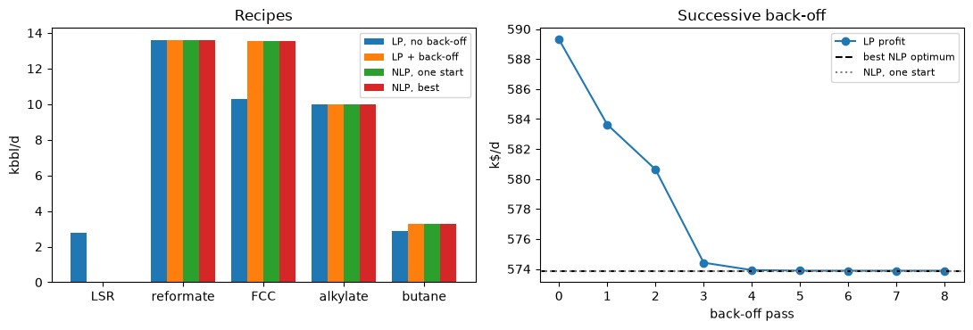
What this shows (on this pool; the numbers move with prices and components):
The unprotected LP over-promises, and its plan is off spec. It reports a margin about 5% (29 k$/d) larger than any feasible plan earns, and in the rigorous pool its recipe misses MON by about 0.6 numbers. Every unit of that error is octane interaction (
linear_blend_error). RVP and sulfur are modelled exactly by the LP rows.A one-shot back-off is not enough. The back-off is a function of the recipe. The first pass, sized at the unprotected plan, still leaves the new plan off spec. It takes about six passes to settle, and the converged back-off (about 0.98 MON) is well above the first estimate (0.58).
The converged back-off reaches the nonlinear optimum here. Every one of the 23 SLSQP starts lands on the same plan, the vertex the back-off loop converges to (reformate and alkylate at availability, no straight-run). That is not guaranteed in general: blending is nonconvex, and the fixed point of successive back-off is a feasible vertex, not a certified optimum. Keep the multistart on a pool with more spread. Coupling the two is what delta-base planning does:
BlendPool.as_block(components)exposes the pool as adifflow.planning.Block, with component volumes as levers and properties and spec margins as outputs.
Caveat. The RT-70 coefficients are the published 75-blend fit as tabulated by Maples (Petroleum Refinery Process Economics, 2nd ed., 2000); the 1959 original was not reachable. An earlier version of this notebook used a MON aromatic coefficient ten times too large, and an olefin×MON interaction where the published form has MON×sensitivity. Both inflated the MON penalty to about two numbers at a spec of 82 (#301). The size of the penalty depends on the coefficients and on how much sensitivity, olefin and aromatic spread the pool carries. Check them against your own blend data before you trust the dollar figures.