
Gradient Checkpointing in JAX#
When differentiating through long computations (deep networks, time-stepping simulations, large flowsheets), memory can become a bottleneck. Gradient checkpointing (also called rematerialization) trades compute for memory by recomputing intermediate values during the backward pass instead of storing them.
Topics covered:
The memory problem in reverse-mode AD
jax.checkpoint(alias:jax.remat) basicsCheckpointing policies
Nested checkpointing strategies
Chemical engineering application: Memory-efficient PFR simulation
import jax
import jax.numpy as jnp
from jax import grad, jit, vmap
from jax import checkpoint, remat  # These are aliases
from functools import partial
import matplotlib.pyplot as plt
import time

jax.config.update("jax_enable_x64", True)

print(f"JAX version: {jax.__version__}")
JAX version: 0.8.2
1. The Memory Problem#
In reverse-mode autodiff (backpropagation), we need intermediate values from the forward pass to compute gradients. For a chain of operations:
The naive approach stores ALL intermediate activations:
\(a_1 = f_1(x)\)
\(a_2 = f_2(a_1)\)
…
\(a_n = f_n(a_{n-1}) = y\)
Memory cost: O(n) - grows linearly with depth!
For a 1000-step PFR simulation with 10 species, this could mean storing 10,000 intermediate arrays.
# Demonstrate the memory issue with a deep computation

def deep_computation(x, n_layers=100):
    """A chain of operations that builds up memory during backprop."""
    for _ in range(n_layers):
        x = jnp.sin(x) + 0.1 * x  # Each layer needs to save x for backward
    return x.sum()

# With large arrays and many layers, memory becomes significant
x = jnp.ones((1000,))

# This works but uses O(n_layers) memory for intermediates
grad_fn = jit(grad(deep_computation))
result = grad_fn(x)

print(f"Input shape: {x.shape}")
print(f"Gradient computed successfully")
print(f"Gradient norm: {jnp.linalg.norm(result):.6f}")
WARNING:2026-01-10 20:31:29,908:jax._src.xla_bridge:852: An NVIDIA GPU may be present on this machine, but a CUDA-enabled jaxlib is not installed. Falling back to cpu.
Input shape: (1000,)
Gradient computed successfully
Gradient norm: 0.000000
2. jax.checkpoint Basics#
jax.checkpoint (or its alias jax.remat) marks a function for rematerialization:
During forward pass: compute normally, but DON’T save intermediates
During backward pass: recompute the forward pass to get needed values
Trade-off: Uses ~2x compute but O(1) memory per checkpointed block.
# Basic checkpoint usage

def expensive_layer(x):
    """A single 'layer' of computation."""
    return jnp.sin(x) + 0.1 * x

# Without checkpointing - saves all intermediates
def deep_no_checkpoint(x, n_layers=100):
    for _ in range(n_layers):
        x = expensive_layer(x)
    return x.sum()

# With checkpointing - recomputes during backward
def deep_with_checkpoint(x, n_layers=100):
    checkpointed_layer = checkpoint(expensive_layer)
    for _ in range(n_layers):
        x = checkpointed_layer(x)
    return x.sum()

x = jnp.ones((1000,))

# Both give the same gradient
grad_no_cp = jit(grad(deep_no_checkpoint))(x)
grad_with_cp = jit(grad(deep_with_checkpoint))(x)

print("Gradient comparison:")
print(f"  Without checkpoint: norm = {jnp.linalg.norm(grad_no_cp):.10f}")
print(f"  With checkpoint:    norm = {jnp.linalg.norm(grad_with_cp):.10f}")
print(f"  Difference: {jnp.linalg.norm(grad_no_cp - grad_with_cp):.2e}")
Gradient comparison:
  Without checkpoint: norm = 0.0000000057
  With checkpoint:    norm = 0.0000000057
  Difference: 0.00e+00
# Using checkpoint as a decorator

@checkpoint
def checkpointed_block(x):
    """This entire block will be recomputed during backprop."""
    x = jnp.sin(x)
    x = jnp.cos(x)
    x = jnp.tanh(x)
    return x

def model(x):
    for _ in range(10):
        x = checkpointed_block(x)
    return x.sum()

x = jnp.ones((100,))
print(f"Gradient with decorated checkpoint: {grad(model)(x)[:5]}...")
Gradient with decorated checkpoint: [9.58528401e-07 9.58528401e-07 9.58528401e-07 9.58528401e-07
 9.58528401e-07]...
3. Checkpointing Policies#
JAX provides fine-grained control over what gets saved vs. recomputed through policies.
Common policies:
everything_saveable: Save nothing, recompute everything (maximum memory savings)nothing_saveable: Save everything (no checkpointing, default behavior)dots_saveable: Save matrix multiplications (expensive to recompute)checkpoint_dots: Recompute everything except dotsCustom policies based on operation type
from jax.ad_checkpoint import checkpoint_policies

# Different policies for different trade-offs

def heavy_computation(x):
    """Mix of cheap (sin) and expensive (matmul) operations."""
    W = jnp.eye(len(x)) * 0.9 + jnp.ones((len(x), len(x))) * 0.01
    x = jnp.sin(x)      # Cheap
    x = W @ x           # Expensive (matrix multiply)
    x = jnp.cos(x)      # Cheap
    x = W.T @ x         # Expensive
    return x

# Policy: save nothing (recompute everything)
recompute_all = checkpoint(
    heavy_computation,
    policy=checkpoint_policies.everything_saveable
)

# Policy: save only matrix multiplies (dots)
save_dots = checkpoint(
    heavy_computation,
    policy=checkpoint_policies.dots_saveable
)

x = jnp.ones((50,))

def loss_fn(layer_fn):
    def loss(x):
        for _ in range(5):
            x = layer_fn(x)
        return x.sum()
    return loss

# All give same gradients
g1 = grad(loss_fn(heavy_computation))(x)
g2 = grad(loss_fn(recompute_all))(x)
g3 = grad(loss_fn(save_dots))(x)

print("Gradient comparison with different policies:")
print(f"  No checkpoint:     {jnp.linalg.norm(g1):.10f}")
print(f"  Recompute all:     {jnp.linalg.norm(g2):.10f}")
print(f"  Save dots only:    {jnp.linalg.norm(g3):.10f}")
Gradient comparison with different policies:
  No checkpoint:     5.9413659024
  Recompute all:     5.9413659024
  Save dots only:    5.9413659024
# Custom checkpoint policy

def custom_policy(prim, *args, **kwargs):
    """
    Custom policy: save expensive operations, recompute cheap ones.

    Returns True if the operation should be SAVED (not recomputed).
    """
    # Save matrix multiplies and convolutions
    expensive_ops = {'dot_general', 'conv_general_dilated'}
    return prim.name in expensive_ops

custom_checkpoint = checkpoint(
    heavy_computation,
    policy=custom_policy
)

g_custom = grad(loss_fn(custom_checkpoint))(x)
print(f"Custom policy gradient: {jnp.linalg.norm(g_custom):.10f}")
Custom policy gradient: 5.9413659024
4. Nested and Hierarchical Checkpointing#
For very deep computations, you can use nested checkpointing with a hierarchical strategy:
Divide computation into blocks
Checkpoint at block level
Within each block, optionally checkpoint at finer granularity
This gives \(O(\sqrt{n})\) memory with \(O(n \log n)\) compute.
# Hierarchical checkpointing for very deep networks

def single_layer(x):
    return jnp.tanh(x * 1.01 + 0.01)

def make_block(n_layers):
    """Create a block of layers with fixed depth."""
    def block(x):
        for _ in range(n_layers):
            x = single_layer(x)
        return x
    return checkpoint(block)

def deep_network_hierarchical(x, n_blocks=10, layers_per_block=10):
    """Total depth = n_blocks * layers_per_block."""
    checkpointed_block = make_block(layers_per_block)
    for _ in range(n_blocks):
        x = checkpointed_block(x)
    return x.sum()

# Compare memory characteristics
# - No checkpoint: O(n_blocks * layers_per_block) memory
# - Block checkpoint: O(n_blocks + layers_per_block) memory

x = jnp.ones((100,))
n_blocks, layers_per_block = 10, 10
total_depth = n_blocks * layers_per_block

grad_result = grad(deep_network_hierarchical)(x, n_blocks, layers_per_block)

print(f"Hierarchical checkpointing:")
print(f"  Total depth: {total_depth} layers")
print(f"  Blocks: {n_blocks}, Layers per block: {layers_per_block}")
print(f"  Memory: O({n_blocks} + {layers_per_block}) = O({n_blocks + layers_per_block})")
print(f"  vs naive O({total_depth})")
print(f"  Gradient norm: {jnp.linalg.norm(grad_result):.6f}")
Hierarchical checkpointing:
  Total depth: 100 layers
  Blocks: 10, Layers per block: 10
  Memory: O(10 + 10) = O(20)
  vs naive O(100)
Gradient norm: 0.000011
5. Checkpointing with jax.lax.scan#
For sequential computations like time-stepping, jax.lax.scan is often used. You can checkpoint the body function to save memory.
from jax import lax

def scan_body(carry, _):
    """One step of a sequential computation."""
    x = carry
    x = jnp.sin(x) + 0.1 * x
    return x, x  # (new_carry, output)

def sequential_no_checkpoint(x, n_steps=100):
    final, trajectory = lax.scan(scan_body, x, None, length=n_steps)
    return final.sum()

# Checkpoint the scan body
checkpointed_body = checkpoint(scan_body)

def sequential_with_checkpoint(x, n_steps=100):
    final, trajectory = lax.scan(checkpointed_body, x, None, length=n_steps)
    return final.sum()

x = jnp.ones((100,))

g1 = grad(sequential_no_checkpoint)(x)
g2 = grad(sequential_with_checkpoint)(x)

print("Scan with checkpointing:")
print(f"  Without checkpoint: gradient norm = {jnp.linalg.norm(g1):.10f}")
print(f"  With checkpoint:    gradient norm = {jnp.linalg.norm(g2):.10f}")
print(f"  Match: {jnp.allclose(g1, g2)}")
Scan with checkpointing:
  Without checkpoint: gradient norm = 0.0000000018
  With checkpoint:    gradient norm = 0.0000000018
  Match: True
6. When to Use Checkpointing#
Use checkpointing when:
Running out of GPU/TPU memory
Deep networks or long time-series
Large batch sizes are needed
Trading ~2x compute for significantly less memory is worthwhile
Don’t use when:
Memory is not a bottleneck
Computation is already slow and memory is fine
Operations are very expensive to recompute (use selective policies)
# Timing comparison

def time_gradient(fn, x, n_runs=10):
    """Time gradient computation."""
    grad_fn = jit(grad(fn))
    # Warmup
    _ = grad_fn(x).block_until_ready()

    times = []
    for _ in range(n_runs):
        start = time.perf_counter()
        _ = grad_fn(x).block_until_ready()
        times.append(time.perf_counter() - start)
    return sum(times) / len(times)

x = jnp.ones((500,))
n_layers = 200

time_no_cp = time_gradient(lambda x: deep_no_checkpoint(x, n_layers), x)
time_with_cp = time_gradient(lambda x: deep_with_checkpoint(x, n_layers), x)

print(f"Timing for {n_layers} layers:")
print(f"  Without checkpoint: {time_no_cp*1000:.2f} ms")
print(f"  With checkpoint:    {time_with_cp*1000:.2f} ms")
print(f"  Slowdown: {time_with_cp/time_no_cp:.2f}x")
print(f"\nNote: ~2x slowdown is expected (forward pass computed twice)")
Timing for 200 layers:
  Without checkpoint: 0.62 ms
  With checkpoint:    0.81 ms
  Slowdown: 1.30x

Note: ~2x slowdown is expected (forward pass computed twice)
7. Chemical Engineering Application: Memory-Efficient PFR#
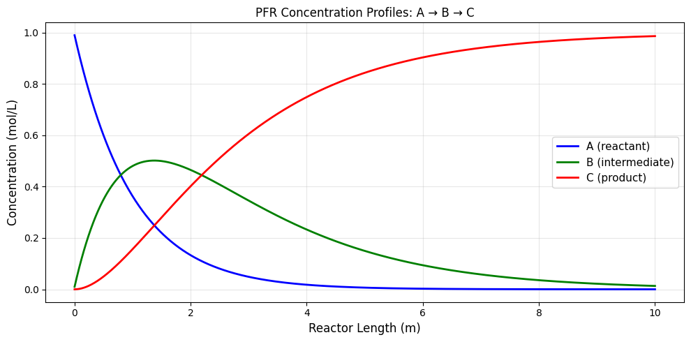
Plug Flow Reactors (PFRs) require integrating ODEs over many steps. For long reactors with many species, memory can be a bottleneck when computing gradients for parameter estimation or optimization.
Scenario: A→B→C consecutive reactions in a PFR
# PFR simulation with gradient checkpointing

def pfr_rates(C, k1, k2):
    """
    A → B → C consecutive first-order reactions.
    C = [C_A, C_B, C_C]
    """
    r1 = k1 * C[0]  # A → B
    r2 = k2 * C[1]  # B → C

    dC_A = -r1
    dC_B = r1 - r2
    dC_C = r2

    return jnp.array([dC_A, dC_B, dC_C])

def euler_step(C, args):
    """Single Euler integration step."""
    k1, k2, dt = args
    dC = pfr_rates(C, k1, k2)
    C_new = C + dt * dC
    return C_new, C_new

# Checkpointed version
euler_step_cp = checkpoint(euler_step)

def simulate_pfr(C0, k1, k2, L, n_steps, use_checkpoint=False):
    """
    Simulate PFR from z=0 to z=L.
    Returns final concentrations.
    """
    dt = L / n_steps
    args = (k1, k2, dt)

    step_fn = euler_step_cp if use_checkpoint else euler_step

    # Use scan for efficient sequential computation
    final_C, trajectory = lax.scan(
        lambda c, _: step_fn(c, args),
        C0,
        None,
        length=n_steps
    )

    return final_C, trajectory

# Initial conditions and parameters
C0 = jnp.array([1.0, 0.0, 0.0])  # Pure A
k1 = 1.0
k2 = 0.5
L = 10.0
n_steps = 1000

# Simulate
final_C, trajectory = simulate_pfr(C0, k1, k2, L, n_steps, use_checkpoint=False)

print("PFR Simulation Results:")
print(f"  Initial: A={C0[0]:.3f}, B={C0[1]:.3f}, C={C0[2]:.3f}")
print(f"  Final:   A={final_C[0]:.6f}, B={final_C[1]:.6f}, C={final_C[2]:.6f}")
print(f"  Mass balance: {final_C.sum():.6f} (should be 1.0)")
PFR Simulation Results:
  Initial: A=1.000, B=0.000, C=0.000
  Final:   A=0.000043, B=0.013222, C=0.986735
Mass balance: 1.000000 (should be 1.0)
# Visualize PFR concentration profiles
z = jnp.linspace(0, L, n_steps)

plt.figure(figsize=(10, 5))
plt.plot(z, trajectory[:, 0], 'b-', label='A (reactant)', linewidth=2)
plt.plot(z, trajectory[:, 1], 'g-', label='B (intermediate)', linewidth=2)
plt.plot(z, trajectory[:, 2], 'r-', label='C (product)', linewidth=2)
plt.xlabel('Reactor Length (m)', fontsize=12)
plt.ylabel('Concentration (mol/L)', fontsize=12)
plt.title('PFR Concentration Profiles: A → B → C', fontsize=12)
plt.legend(fontsize=11)
plt.grid(True, alpha=0.3)
plt.tight_layout()
plt.show()
# Gradient computation: optimize k1, k2 to maximize B at outlet

def objective(params, use_checkpoint=False):
    """Objective: Maximize B concentration at reactor outlet."""
    k1, k2 = params
    final_C, _ = simulate_pfr(C0, k1, k2, L, n_steps, use_checkpoint)
    return -final_C[1]  # Negative because we minimize

# Compare gradients with and without checkpointing
params = jnp.array([1.0, 0.5])

grad_no_cp = grad(lambda p: objective(p, use_checkpoint=False))(params)
grad_with_cp = grad(lambda p: objective(p, use_checkpoint=True))(params)

print("Gradients for PFR optimization:")
print(f"  ∂(-C_B)/∂k1 = {grad_no_cp[0]:.6f} (no checkpoint)")
print(f"  ∂(-C_B)/∂k1 = {grad_with_cp[0]:.6f} (with checkpoint)")
print(f"  ∂(-C_B)/∂k2 = {grad_no_cp[1]:.6f} (no checkpoint)")
print(f"  ∂(-C_B)/∂k2 = {grad_with_cp[1]:.6f} (with checkpoint)")
print(f"\nGradients match: {jnp.allclose(grad_no_cp, grad_with_cp)}")
Gradients for PFR optimization:
  ∂(-C_B)/∂k1 = 0.012349 (no checkpoint)
  ∂(-C_B)/∂k1 = 0.012349 (with checkpoint)
  ∂(-C_B)/∂k2 = 0.107305 (no checkpoint)
  ∂(-C_B)/∂k2 = 0.107305 (with checkpoint)

Gradients match: True
# Memory scaling comparison
# Note: We can't easily measure memory in JAX, but we can reason about it

print("Memory Analysis for PFR Gradient Computation")
print("=" * 50)
print(f"\nScenario: {n_steps} integration steps, 3 species")
print(f"")
print("Without checkpointing:")
print(f"  Must store: {n_steps} × 3 = {n_steps * 3} intermediate values")
print(f"  Memory: O(n_steps × n_species)")
print(f"")
print("With checkpointing (per-step):")
print(f"  Must store: Only current state (3 values)")
print(f"  Memory: O(n_species)")
print(f"  Trade-off: ~2× compute time")
print(f"")
print("With hierarchical checkpointing (blocks of 100 steps):")
n_blocks = n_steps // 100
print(f"  Must store: {n_blocks} block boundaries + 100 steps within block")
print(f"  Memory: O(n_blocks + steps_per_block) = O({n_blocks + 100})")
print(f"  Better compute/memory trade-off for very long simulations")
Memory Analysis for PFR Gradient Computation
==================================================

Scenario: 1000 integration steps, 3 species

Without checkpointing:
  Must store: 1000 × 3 = 3000 intermediate values
  Memory: O(n_steps × n_species)

With checkpointing (per-step):
  Must store: Only current state (3 values)
  Memory: O(n_species)
  Trade-off: ~2× compute time

With hierarchical checkpointing (blocks of 100 steps):
  Must store: 10 block boundaries + 100 steps within block
  Memory: O(n_blocks + steps_per_block) = O(110)
  Better compute/memory trade-off for very long simulations
# Gradient-based optimization of rate constants
import optax

# Target: find k1, k2 that maximize intermediate B
@jit
def loss_and_grad(params):
    return jax.value_and_grad(lambda p: objective(p, use_checkpoint=True))(params)

# Simple gradient descent
params = jnp.array([0.5, 0.3])  # Initial guess
learning_rate = 0.1

optimizer = optax.adam(learning_rate)
opt_state = optimizer.init(params)

print("Optimizing rate constants to maximize intermediate B:")
print(f"{'Iteration':<10} {'k1':<10} {'k2':<10} {'C_B':<10}")
print("-" * 40)

for i in range(50):
    loss, grads = loss_and_grad(params)
    updates, opt_state = optimizer.update(grads, opt_state)
    params = optax.apply_updates(params, updates)

    # Keep parameters positive
    params = jnp.maximum(params, 0.01)

    if i % 10 == 0 or i == 49:
        C_B = -loss
        print(f"{i:<10} {params[0]:<10.4f} {params[1]:<10.4f} {C_B:<10.6f}")

print(f"\nOptimal: k1={params[0]:.4f}, k2={params[1]:.4f}")
print(f"Maximum B concentration: {-objective(params, use_checkpoint=True):.6f}")
Optimizing rate constants to maximize intermediate B:
Iteration  k1         k2         C_B
----------------------------------------
0          0.4000     0.2000     0.107273
10         0.6240     0.0100     0.917683
20         0.8598     0.0100     0.915442
30         0.9231     0.0100     0.914671
40         0.9187     0.0100     0.914670
49         0.8885     0.0100     0.914955

Optimal: k1=0.8885, k2=0.0100
Maximum B concentration: 0.914998
8. Advanced: Checkpointing with Diffrax#
When using diffrax for ODE solving, checkpointing is handled through adjoint methods. The RecursiveCheckpointAdjoint provides memory-efficient gradient computation.
import diffrax

def pfr_dynamics(t, C, args):
    """ODE right-hand side for PFR."""
    k1, k2 = args
    return pfr_rates(C, k1, k2)

def solve_pfr_diffrax(params, C0, t_span, adjoint_type='recursive'):
    """Solve PFR using diffrax with different adjoint methods."""
    k1, k2 = params

    term = diffrax.ODETerm(pfr_dynamics)
    solver = diffrax.Tsit5()  # 5th order Runge-Kutta

    # Choose adjoint method
    if adjoint_type == 'recursive':
        # Memory-efficient: O(log(n)) memory
        adjoint = diffrax.RecursiveCheckpointAdjoint()
    elif adjoint_type == 'backsolve':
        # Solves adjoint ODE backward in time
        adjoint = diffrax.BacksolveAdjoint()
    else:
        # Direct: stores all steps (memory intensive)
        adjoint = diffrax.DirectAdjoint()

    solution = diffrax.diffeqsolve(
        term, solver,
        t0=t_span[0], t1=t_span[1],
        dt0=0.01,
        y0=C0,
        args=(k1, k2),
        adjoint=adjoint,
        saveat=diffrax.SaveAt(t1=True)
    )

    return solution.ys[-1]

# Compare adjoint methods
params = jnp.array([1.0, 0.5])
C0 = jnp.array([1.0, 0.0, 0.0])
t_span = (0.0, 10.0)

def objective_diffrax(params, adjoint_type):
    C_final = solve_pfr_diffrax(params, C0, t_span, adjoint_type)
    return -C_final[1]  # Maximize B

print("Diffrax Adjoint Methods Comparison:")
print("=" * 50)

for adj in ['recursive', 'backsolve', 'direct']:
    grad_val = grad(lambda p: objective_diffrax(p, adj))(params)
    obj_val = -objective_diffrax(params, adj)
    print(f"\n{adj.capitalize()} adjoint:")
    print(f"  C_B at outlet: {obj_val:.6f}")
    print(f"  ∂C_B/∂k1 = {-grad_val[0]:.6f}")
    print(f"  ∂C_B/∂k2 = {-grad_val[1]:.6f}")
Diffrax Adjoint Methods Comparison:
==================================================
Recursive adjoint:
  C_B at outlet: 0.013385
  ∂C_B/∂k1 = -0.012477
  ∂C_B/∂k2 = -0.107989
Backsolve adjoint:
  C_B at outlet: 0.013385
  ∂C_B/∂k1 = -0.012477
  ∂C_B/∂k2 = -0.107989
Direct adjoint:
  C_B at outlet: 0.013385
  ∂C_B/∂k1 = -0.012477
  ∂C_B/∂k2 = -0.107989
Summary#
Key concepts:
The memory problem: Reverse-mode AD stores O(n) intermediates for depth-n computations
jax.checkpoint/jax.remat: Trades ~2x compute for O(1) memory per blockPolicies: Fine-grained control over what to save vs. recompute
everything_saveable: Maximum memory savingsdots_saveable: Save expensive matmulsCustom policies for specific needs
Hierarchical checkpointing: O(√n) memory with O(n log n) compute
With
lax.scan: Checkpoint the body function for sequential computationsWith diffrax: Use
RecursiveCheckpointAdjointfor memory-efficient ODE gradients
When to use:
Long time-series simulations (PFR, dynamic models)
Deep neural networks
Large batch training
GPU/TPU memory constraints
Chemical engineering applications:
Parameter estimation in PFRs
Dynamic process optimization
Training surrogate models on long trajectories
Sensitivity analysis of multi-step processes