
Technoeconomic Analysis with Differentiable Flowsheets#
This notebook demonstrates comprehensive Technoeconomic Analysis (TEA) integrated with JAX-based process simulation. All calculations are fully differentiable, enabling gradient-based optimization of process economics.
What You’ll Learn#
Equipment Sizing & Capital Costs - Cost correlations for reactors, heat exchangers, etc.
Operating Costs - Utilities, raw materials, labor, maintenance
Profitability Metrics - NPV, IRR, MSP, payback period
Gradient-Based Optimization - Maximize profit using autodiff
Sensitivity Analysis - Understand how parameters affect economics
Process Overview#
We analyze a simple CSTR process:
Reaction: A → B (first-order, exothermic)
Design Variables: Reactor volume (V), Temperature (T)
Objective: Maximize annual profit
import jax
import jax.numpy as jnp
from jax import Array
jax.config.update("jax_enable_x64", True)

# Process simulation imports
from difflow.streams import make_stream, get_flows
from difflow.thermo import IdealThermo, SpeciesData
from difflow.units.cstr import CSTR, CSTRParams

# Economics imports
import difflow.economics as econ

print("Imports successful!")
WARNING:2026-03-01 07:49:20,899:jax._src.xla_bridge:905: Platform 'METAL' is experimental and not all JAX functionality may be correctly supported!
WARNING: All log messages before absl::InitializeLog() is called are written to STDERR
W0000 00:00:1772369360.899558 12635422 mps_client.cc:510] WARNING: JAX Apple GPU support is experimental and not all JAX functionality is correctly supported!
I0000 00:00:1772369360.909451 12635422 service.cc:145] XLA service 0xa73513300 initialized for platform METAL (this does not guarantee that XLA will be used). Devices:
I0000 00:00:1772369360.909460 12635422 service.cc:153]   StreamExecutor device (0): Metal, <undefined>
I0000 00:00:1772369360.910444 12635422 mps_client.cc:406] Using Simple allocator.
I0000 00:00:1772369360.910453 12635422 mps_client.cc:384] XLA backend will use up to 55662313472 bytes on device 0 for SimpleAllocator.
WARNING:2026-03-01 07:49:20,910:jax._src.xla_bridge:905: Platform 'mps' is experimental and not all JAX functionality may be correctly supported!
Metal device set to: Apple M4 Pro
Imports successful!
1. Process Setup#
Define the reaction system: A → B with Arrhenius kinetics
where:
\(A = 10^6\) s⁻¹ (pre-exponential factor)
\(E_a = 50\) kJ/mol (activation energy)
\(\Delta H_{rxn} = -50\) kJ/mol (exothermic)
# Define species thermodynamic properties
species_data = {
    "A": SpeciesData(
        name="A", MW=100.0, Cp_coeffs=(75.0, 0.0, 0.0, 0.0),
        Hvap_coeffs=(35000.0, 0.38, 500.0), antoine_coeffs=(10.0, 3000.0, -50.0),
        Hf=0.0,
    ),
    "B": SpeciesData(
        name="B", MW=100.0, Cp_coeffs=(75.0, 0.0, 0.0, 0.0),
        Hvap_coeffs=(30000.0, 0.38, 450.0), antoine_coeffs=(10.0, 2800.0, -40.0),
        Hf=-50000.0,  # Exothermic reaction
    ),
}

thermo = IdealThermo(species_data)
species_order = ["A", "B"]
stoichiometry = jnp.array([[-1.0], [+1.0]])  # A consumed, B produced

def rate_function(C: dict[str, Array], T: Array, params: dict) -> Array:
    """First-order reaction: A → B with Arrhenius kinetics."""
    k = params["A"] * jnp.exp(-params["Ea"] / (8.314 * T))
    return jnp.array([k * C["A"]])

# Kinetic parameters
kinetic_params = {
    "A": jnp.array(1e6),      # Pre-exponential (1/s)
    "Ea": jnp.array(50000.0),  # Activation energy (J/mol)
}

print("Process setup complete!")
print(f"  Pre-exponential factor: {float(kinetic_params['A']):.0e} 1/s")
print(f"  Activation energy: {float(kinetic_params['Ea'])/1000:.0f} kJ/mol")
Process setup complete!
  Pre-exponential factor: 1e+06 1/s
  Activation energy: 50 kJ/mol
2. Integrated Process Economics Model#
We create a class that combines process simulation with economic calculations. This enables computing profit, NPV, and other metrics as differentiable functions of design variables.
class ProcessEconomics:
    """Integrated process simulation with economics.

    All methods are JAX-differentiable for optimization.
    """

    def __init__(
        self,
        feed_rate: float = 10.0,  # mol/s of A
        feed_temp: float = 300.0,  # K
        prices: dict | None = None,
    ):
        self.feed_rate = feed_rate
        self.feed_temp = feed_temp

        # Economic parameters
        self.prices = prices or {
            "A": 50.0,   # $/kmol raw material A
            "B": 200.0,  # $/kmol product B
        }

        # Operating parameters
        self.hours_per_year = 8000.0
        self.seconds_per_year = self.hours_per_year * 3600.0

    def simulate(self, V: Array, T: Array) -> tuple[dict, dict]:
        """Run reactor simulation."""
        params = CSTRParams(
            V=V,
            rate_fn=rate_function,
            stoich=stoichiometry,
            rate_params=kinetic_params,
            species_order=species_order,
            dH_rxn=jnp.array([-50000.0]),
        )
        cstr = CSTR(params, thermo=thermo, mode="isothermal")

        inlet = make_stream(
            {"A": self.feed_rate, "B": 0.0},
            T=self.feed_temp,
            P=101325.0
        )

        outlet, info = cstr(inlet, T_spec=T)
        return outlet, info

    def capital_cost(self, V: Array) -> dict[str, Array]:
        """Calculate capital costs."""
        # Reactor cost (jacketed CSTR)
        reactor_purchased = econ.reactor_cost(V, "cstr_jacketed")

        # Installed costs with Lang factor
        reactor_installed = econ.installed_cost(reactor_purchased, lang_factor=4.74)

        # Auxiliary equipment (pumps, piping) = 30% of reactor
        auxiliary = reactor_installed * 0.30
        total_installed = reactor_installed + auxiliary

        # Working capital = 15% of FCI
        working_capital = total_installed * 0.15

        return {
            "reactor_purchased": reactor_purchased,
            "reactor_installed": reactor_installed,
            "auxiliary": auxiliary,
            "total_installed": total_installed,
            "working_capital": working_capital,
            "total_capital": total_installed + working_capital,
        }

    def operating_cost(self, V: Array, T: Array, outlet: dict, info: dict) -> dict[str, Array]:
        """Calculate operating costs ($/year)."""
        # Raw material cost
        raw_material_per_s = self.feed_rate * self.prices["A"] / 1000  # $/s
        raw_material_annual = raw_material_per_s * self.seconds_per_year

        # Utility cost (cooling for exothermic reaction)
        Q = jnp.abs(info["Q"])  # Heat duty (W)
        utility_per_s = econ.cooling_water_cost(Q)
        utility_annual = utility_per_s * self.seconds_per_year

        # Labor, maintenance, overhead (from FCI)
        capex = self.capital_cost(V)
        fci = capex["total_installed"]

        labor_annual = fci * 0.02       # 2% of FCI
        maintenance_annual = fci * 0.04  # 4% of FCI
        overhead_annual = fci * 0.02     # 2% of FCI

        total_opex = (
            raw_material_annual + utility_annual +
            labor_annual + maintenance_annual + overhead_annual
        )

        return {
            "raw_materials": raw_material_annual,
            "utilities": utility_annual,
            "labor": labor_annual,
            "maintenance": maintenance_annual,
            "overhead": overhead_annual,
            "total_opex": total_opex,
        }

    def revenue(self, outlet: dict) -> dict[str, Array]:
        """Calculate annual revenue ($/year)."""
        F_B_out = outlet["F_B"]  # mol/s
        revenue_per_s = F_B_out * self.prices["B"] / 1000  # $/s
        revenue_annual = revenue_per_s * self.seconds_per_year

        return {"product_revenue": revenue_annual}

    def annual_profit(self, V: Array, T: Array) -> Array:
        """Calculate annual profit (differentiable)."""
        outlet, info = self.simulate(V, T)

        capex = self.capital_cost(V)
        opex = self.operating_cost(V, T, outlet, info)
        rev = self.revenue(outlet)

        # Annualized capital cost (10% discount rate, 20 year life)
        crf = econ.capital_recovery_factor(jnp.array(0.10), jnp.array(20.0))
        annual_capex = capex["total_capital"] * crf

        profit = rev["product_revenue"] - opex["total_opex"] - annual_capex
        return profit

    def npv(self, V: Array, T: Array, discount_rate: float = 0.10, plant_life: int = 20) -> Array:
        """Calculate Net Present Value."""
        outlet, info = self.simulate(V, T)

        capex = self.capital_cost(V)
        opex = self.operating_cost(V, T, outlet, info)
        rev = self.revenue(outlet)

        # Annual cash flow
        annual_cf = rev["product_revenue"] - opex["total_opex"]
        cash_flows = jnp.ones(plant_life) * annual_cf

        # Add working capital recovery in final year
        cash_flows = cash_flows.at[-1].add(capex["working_capital"])

        return econ.npv(cash_flows, jnp.array(discount_rate), capex["total_capital"])

    def minimum_selling_price(self, V: Array, T: Array) -> Array:
        """Calculate minimum selling price for breakeven ($/kmol)."""
        outlet, info = self.simulate(V, T)

        capex = self.capital_cost(V)
        opex = self.operating_cost(V, T, outlet, info)

        # Annualized capital
        crf = econ.capital_recovery_factor(jnp.array(0.10), jnp.array(20.0))
        annual_capex = capex["total_capital"] * crf

        total_annual_cost = opex["total_opex"] + annual_capex

        # Annual production of B
        F_B_out = outlet["F_B"]  # mol/s
        annual_production = F_B_out * self.seconds_per_year / 1000  # kmol/year

        return total_annual_cost / jnp.maximum(annual_production, 1e-10)

print("ProcessEconomics class defined!")
ProcessEconomics class defined!
3. Basic Technoeconomic Analysis#
Let’s analyze a base case design with V = 2 m³ and T = 400 K.
pe = ProcessEconomics()

# Base case design
V = jnp.array(2.0)   # m³
T = jnp.array(400.0)  # K

print(f"Base Case: V = {float(V):.1f} m³, T = {float(T):.0f} K")
print("=" * 50)

# Simulate
outlet, info = pe.simulate(V, T)
conversion = float(info["conversion"]["A"]) * 100
print(f"\nProcess Performance:")
print(f"  Conversion: {conversion:.1f}%")
print(f"  Heat duty: {float(info['Q'])/1000:.1f} kW (cooling required)")
print(f"  Product rate: {float(outlet['F_B']):.2f} mol/s = {float(outlet['F_B'])*3600/1000:.1f} kmol/hr")
Base Case: V = 2.0 m³, T = 400 K
==================================================
Process Performance:
  Conversion: 100.0%
  Heat duty: -424.8 kW (cooling required)
  Product rate: 10.00 mol/s = 36.0 kmol/hr
# Capital costs breakdown
capex = pe.capital_cost(V)

print("Capital Costs:")
print("-" * 50)
print(f"  Reactor (purchased):   ${float(capex['reactor_purchased']):>12,.0f}")
print(f"  Reactor (installed):   ${float(capex['reactor_installed']):>12,.0f}")
print(f"  Auxiliary equipment:   ${float(capex['auxiliary']):>12,.0f}")
print(f"  Working capital:       ${float(capex['working_capital']):>12,.0f}")
print("-" * 50)
print(f"  TOTAL CAPITAL:         ${float(capex['total_capital']):>12,.0f}")
Capital Costs:
--------------------------------------------------
  Reactor (purchased):   $      23,101
  Reactor (installed):   $     109,499
  Auxiliary equipment:   $      32,850
  Working capital:       $      21,352
--------------------------------------------------
  TOTAL CAPITAL:         $     163,701
# Operating costs breakdown
opex = pe.operating_cost(V, T, outlet, info)

print("Operating Costs ($/year):")
print("-" * 50)
print(f"  Raw materials:         ${float(opex['raw_materials']):>12,.0f}")
print(f"  Utilities:             ${float(opex['utilities']):>12,.0f}")
print(f"  Labor:                 ${float(opex['labor']):>12,.0f}")
print(f"  Maintenance:           ${float(opex['maintenance']):>12,.0f}")
print(f"  Overhead:              ${float(opex['overhead']):>12,.0f}")
print("-" * 50)
print(f"  TOTAL OPEX:            ${float(opex['total_opex']):>12,.0f}")
Operating Costs ($/year):
--------------------------------------------------
  Raw materials:         $  14,400,000
  Utilities:             $       4,282
  Labor:                 $       2,847
  Maintenance:           $       5,694
  Overhead:              $       2,847
--------------------------------------------------
  TOTAL OPEX:            $  14,415,670
# Revenue and profitability
rev = pe.revenue(outlet)
profit = pe.annual_profit(V, T)
npv_val = pe.npv(V, T)
msp = pe.minimum_selling_price(V, T)

print("Revenue & Profitability:")
print("-" * 50)
print(f"  Product B sales:       ${float(rev['product_revenue']):>12,.0f}/year")
print(f"  Annual Profit:         ${float(profit):>12,.0f}/year")
print(f"  NPV (10%, 20yr):       ${float(npv_val):>12,.0f}")
print(f"  MSP (breakeven):       ${float(msp):>12.2f}/kmol")
print(f"  Current price:         ${pe.prices['B']:>12.2f}/kmol")
print(f"  Margin:                ${pe.prices['B'] - float(msp):>12.2f}/kmol")
Revenue & Profitability:
--------------------------------------------------
  Product B sales:       $  57,582,440/year
  Annual Profit:         $  43,147,541/year
  NPV (10%, 20yr):       $ 367,342,513
  MSP (breakeven):       $       50.14/kmol
  Current price:         $      200.00/kmol
  Margin:                $      149.86/kmol
4. Equipment Cost Correlations#
The difflow.economics module provides cost correlations for various equipment types, all updated to 2024 dollars using CEPCI indices.
print("Reactor Costs (2024 $, installed with Lang factor 4.74):")
print("-" * 60)
print(f"{'Volume (m³)':>12} {'Purchased ($)':>15} {'Installed ($)':>15}")
print("-" * 60)
for V_val in [0.5, 1.0, 2.0, 5.0, 10.0]:
    purchased = econ.reactor_cost(jnp.array(V_val), "cstr_jacketed")
    installed = econ.installed_cost(purchased)
    print(f"{V_val:>12.1f} {float(purchased):>15,.0f} {float(installed):>15,.0f}")
Reactor Costs (2024 $, installed with Lang factor 4.74):
------------------------------------------------------------
 Volume (m³)   Purchased ($)   Installed ($)
------------------------------------------------------------
         0.5          22,971         108,884
         1.0          23,018         109,103
         2.0          23,101         109,499
         5.0          23,322         110,547
        10.0          23,650         112,101
print("\nHeat Exchanger Costs (Shell & Tube, Floating Head):")
print("-" * 60)
print(f"{'Area (m²)':>12} {'Purchased ($)':>15} {'Installed ($)':>15}")
print("-" * 60)
for A_val in [10, 50, 100, 500, 1000]:
    purchased = econ.heat_exchanger_cost(jnp.array(float(A_val)), "shell_tube_floating")
    installed = econ.installed_cost(purchased)
    print(f"{A_val:>12d} {float(purchased):>15,.0f} {float(installed):>15,.0f}")
Heat Exchanger Costs (Shell & Tube, Floating Head):
------------------------------------------------------------
   Area (m²)   Purchased ($)   Installed ($)
------------------------------------------------------------
          10          16,268          77,111
          50          19,167          90,853
         100          21,582         102,297
         500          33,124         157,007
        1000          42,736         202,568
print("\nMaterial Factors (for 2 m³ CSTR):")
print("-" * 50)
base_cost = econ.reactor_cost(jnp.array(2.0), "cstr_jacketed")
print(f"{'Material':15} {'Factor':>8} {'Cost ($)':>15}")
print("-" * 50)
for material, factor in [
    ("Carbon Steel", 1.0),
    ("Stainless 304", 1.8),
    ("Stainless 316", 2.1),
    ("Hastelloy C", 4.0),
    ("Titanium", 7.0),
]:
    adjusted = base_cost * factor
    print(f"{material:15} {factor:>8.1f} {float(adjusted):>15,.0f}")
Material Factors (for 2 m³ CSTR):
--------------------------------------------------
Material          Factor        Cost ($)
--------------------------------------------------
Carbon Steel         1.0          23,101
Stainless 304        1.8          41,582
Stainless 316        2.1          48,512
Hastelloy C          4.0          92,404
Titanium             7.0         161,708
5. Gradient-Based Profit Optimization#
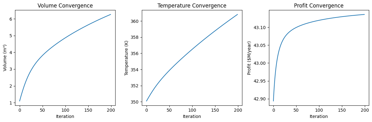
Because all calculations are JAX-differentiable, we can use gradient descent to find the optimal reactor design that maximizes profit.
import optax

pe = ProcessEconomics()

# Objective: maximize profit (minimize negative profit)
def neg_profit(params: Array) -> Array:
    V, T = params[0], params[1]
    return -pe.annual_profit(V, T)

# Gradient function
grad_fn = jax.grad(neg_profit)

# Initial guess
x = jnp.array([1.0, 350.0])
print(f"Initial: V = {x[0]:.2f} m³, T = {x[1]:.0f} K")
print(f"Initial profit: ${-float(neg_profit(x)):,.0f}/year")

# Check initial gradients
g = grad_fn(x)
print(f"Initial gradients: ∂profit/∂V = ${float(-g[0]):,.0f}/m³, ∂profit/∂T = ${float(-g[1]):,.0f}/K")
print("(Positive gradients → increasing V and T increases profit)")

# Use Adam optimizer with appropriate learning rate
# Adam adapts step sizes based on gradient history
optimizer = optax.adam(learning_rate=0.1)
opt_state = optimizer.init(x)

print("\nOptimizing with Adam...")
print("-" * 70)
history = []
n_iters = 200
for i in range(n_iters):
    grad = grad_fn(x)
    updates, opt_state = optimizer.update(grad, opt_state, x)
    x = optax.apply_updates(x, updates)

    # Apply bounds (reasonable reactor limits)
    x = jnp.clip(x, jnp.array([0.1, 300.0]), jnp.array([10.0, 500.0]))

    profit = -neg_profit(x)
    history.append((float(x[0]), float(x[1]), float(profit)))

    if (i + 1) % 20 == 0:
        at_bound = ""
        if x[0] >= 9.9 and x[1] >= 499:
            at_bound = " [at boundary]"
        print(f"  Iter {i+1:3d}: V = {x[0]:.2f} m³, T = {x[1]:.0f} K, Profit = ${float(profit):,.0f}/year{at_bound}")

V_opt, T_opt = float(x[0]), float(x[1])

print("\nNote: The optimizer converges to the upper bounds because:")
print("  - Higher temperature increases reaction rate → more product")
print("  - Larger volume increases residence time → higher conversion")
print("  - The cost increase is small compared to the revenue increase")
print("  - In practice, there would be safety/material limits on T")
Initial: V = 1.00 m³, T = 350 K
Initial profit: $42,865,476/year
Initial gradients: ∂profit/∂V = $297,684/m³, ∂profit/∂T = $14,628/K
(Positive gradients → increasing V and T increases profit)

Optimizing with Adam...
----------------------------------------------------------------------
Iter 20: V = 2.61 m³, T = 352 K, Profit = $43,059,363/year
Iter 40: V = 3.49 m³, T = 353 K, Profit = $43,090,902/year
Iter 60: V = 4.04 m³, T = 354 K, Profit = $43,104,481/year
Iter 80: V = 4.48 m³, T = 355 K, Profit = $43,112,940/year
Iter 100: V = 4.85 m³, T = 356 K, Profit = $43,119,065/year
Iter 120: V = 5.18 m³, T = 357 K, Profit = $43,123,808/year
Iter 140: V = 5.48 m³, T = 358 K, Profit = $43,127,622/year
Iter 160: V = 5.76 m³, T = 359 K, Profit = $43,130,769/year
Iter 180: V = 6.02 m³, T = 360 K, Profit = $43,133,419/year
  Iter 200: V = 6.26 m³, T = 361 K, Profit = $43,135,684/year

Note: The optimizer converges to the upper bounds because:
  - Higher temperature increases reaction rate → more product
  - Larger volume increases residence time → higher conversion
  - The cost increase is small compared to the revenue increase
  - In practice, there would be safety/material limits on T
# Final optimized results
print("\nOptimal Design:")
print("=" * 50)
print(f"  Volume: {V_opt:.2f} m³")
print(f"  Temperature: {T_opt:.0f} K")

outlet_opt, info_opt = pe.simulate(jnp.array(V_opt), jnp.array(T_opt))
print(f"  Conversion: {float(info_opt['conversion']['A'])*100:.1f}%")
print(f"  Annual Profit: ${float(pe.annual_profit(jnp.array(V_opt), jnp.array(T_opt))):,.0f}")
print(f"  NPV: ${float(pe.npv(jnp.array(V_opt), jnp.array(T_opt))):,.0f}")
Optimal Design:
==================================================
  Volume: 6.26 m³
  Temperature: 361 K
  Conversion: 100.0%
  Annual Profit: $43,135,684
  NPV: $367,241,612
# Visualize optimization trajectory
import matplotlib.pyplot as plt

fig, axes = plt.subplots(1, 3, figsize=(12, 4))

V_hist = [h[0] for h in history]
T_hist = [h[1] for h in history]
profit_hist = [h[2] for h in history]

axes[0].plot(V_hist)
axes[0].set_xlabel('Iteration')
axes[0].set_ylabel('Volume (m³)')
axes[0].set_title('Volume Convergence')

axes[1].plot(T_hist)
axes[1].set_xlabel('Iteration')
axes[1].set_ylabel('Temperature (K)')
axes[1].set_title('Temperature Convergence')

axes[2].plot([p/1e6 for p in profit_hist])
axes[2].set_xlabel('Iteration')
axes[2].set_ylabel('Profit ($M/year)')
axes[2].set_title('Profit Convergence')

plt.tight_layout()
plt.show()
6. Sensitivity Analysis#
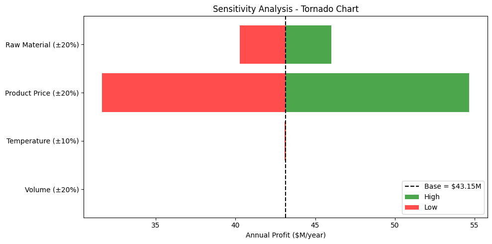
Gradients tell us how sensitive the economics are to design changes. This is valuable for understanding which parameters matter most.
pe = ProcessEconomics()

# Base case
V = jnp.array(2.0)
T = jnp.array(400.0)

print(f"Base Case: V = {float(V):.1f} m³, T = {float(T):.0f} K")
print("=" * 50)

# Calculate gradients of profit w.r.t. design variables
def profit_fn(V, T):
    return pe.annual_profit(V, T)

grad_V = jax.grad(profit_fn, argnums=0)(V, T)
grad_T = jax.grad(profit_fn, argnums=1)(V, T)

print(f"\nProfit Sensitivities:")
print(f"  ∂Profit/∂V = ${float(grad_V):,.0f} per m³")
print(f"  ∂Profit/∂T = ${float(grad_T):,.0f} per K")

# NPV sensitivities
def npv_fn(V, T):
    return pe.npv(V, T)

grad_npv_V = jax.grad(npv_fn, argnums=0)(V, T)
grad_npv_T = jax.grad(npv_fn, argnums=1)(V, T)

print(f"\nNPV Sensitivities:")
print(f"  ∂NPV/∂V = ${float(grad_npv_V):,.0f} per m³")
print(f"  ∂NPV/∂T = ${float(grad_npv_T):,.0f} per K")
Base Case: V = 2.0 m³, T = 400 K
==================================================
Profit Sensitivities:
  ∂Profit/∂V = $8,671 per m³
  ∂Profit/∂T = $667 per K
NPV Sensitivities:
  ∂NPV/∂V = $73,833 per m³
  ∂NPV/∂T = $5,681 per K
# Sensitivity to product price
print("\nSensitivity to Product Price:")
print("-" * 50)

base_profit = profit_fn(V, T)
price_data = []

for price_mult in [0.8, 0.9, 1.0, 1.1, 1.2]:
    pe_temp = ProcessEconomics(prices={"A": 50.0, "B": 200.0 * price_mult})
    profit = pe_temp.annual_profit(V, T)
    change = (float(profit) - float(base_profit)) / float(base_profit) * 100
    price_data.append((200*price_mult, float(profit), change))
    print(f"  B price = ${200*price_mult:.0f}/kmol: Profit = ${float(profit):>10,.0f} ({change:+.1f}%)")
Sensitivity to Product Price:
--------------------------------------------------
  B price = $160/kmol: Profit = $31,631,053 (-26.7%)
  B price = $180/kmol: Profit = $37,389,297 (-13.3%)
  B price = $200/kmol: Profit = $43,147,541 (+0.0%)
  B price = $220/kmol: Profit = $48,905,785 (+13.3%)
B price = $240/kmol: Profit = $54,664,029 (+26.7%)
# Tornado chart of sensitivities
fig, ax = plt.subplots(figsize=(10, 5))

# Calculate normalized sensitivities
base_V, base_T = 2.0, 400.0
base_profit_val = float(pe.annual_profit(jnp.array(base_V), jnp.array(base_T)))

sensitivities = []

# Volume ±20%
profit_low = float(pe.annual_profit(jnp.array(base_V * 0.8), jnp.array(base_T)))
profit_high = float(pe.annual_profit(jnp.array(base_V * 1.2), jnp.array(base_T)))
sensitivities.append(('Volume (±20%)', profit_low/1e6, profit_high/1e6))

# Temperature ±10%
profit_low = float(pe.annual_profit(jnp.array(base_V), jnp.array(base_T * 0.9)))
profit_high = float(pe.annual_profit(jnp.array(base_V), jnp.array(base_T * 1.1)))
sensitivities.append(('Temperature (±10%)', profit_low/1e6, profit_high/1e6))

# Product price ±20%
pe_low = ProcessEconomics(prices={"A": 50.0, "B": 160.0})
pe_high = ProcessEconomics(prices={"A": 50.0, "B": 240.0})
profit_low = float(pe_low.annual_profit(jnp.array(base_V), jnp.array(base_T)))
profit_high = float(pe_high.annual_profit(jnp.array(base_V), jnp.array(base_T)))
sensitivities.append(('Product Price (±20%)', profit_low/1e6, profit_high/1e6))

# Raw material price ±20%
pe_low = ProcessEconomics(prices={"A": 40.0, "B": 200.0})
pe_high = ProcessEconomics(prices={"A": 60.0, "B": 200.0})
profit_low = float(pe_low.annual_profit(jnp.array(base_V), jnp.array(base_T)))
profit_high = float(pe_high.annual_profit(jnp.array(base_V), jnp.array(base_T)))
sensitivities.append(('Raw Material (±20%)', profit_high/1e6, profit_low/1e6))  # Note: reversed

# Plot
base_profit_M = base_profit_val / 1e6
labels = [s[0] for s in sensitivities]
y_pos = range(len(labels))

for i, (label, low, high) in enumerate(sensitivities):
    ax.barh(i, high - base_profit_M, left=base_profit_M, color='green', alpha=0.7, label='High' if i==0 else '')
    ax.barh(i, low - base_profit_M, left=base_profit_M, color='red', alpha=0.7, label='Low' if i==0 else '')

ax.axvline(x=base_profit_M, color='black', linestyle='--', label=f'Base = ${base_profit_M:.2f}M')
ax.set_yticks(y_pos)
ax.set_yticklabels(labels)
ax.set_xlabel('Annual Profit ($M/year)')
ax.set_title('Sensitivity Analysis - Tornado Chart')
ax.legend(loc='lower right')
plt.tight_layout()
plt.show()
7. Process Alternatives Comparison#
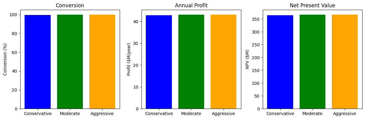
Compare different design philosophies: conservative, moderate, and aggressive.
alternatives = [
    ("Conservative", 1.0, 350.0),
    ("Moderate", 2.0, 400.0),
    ("Aggressive", 4.0, 450.0),
]

pe = ProcessEconomics()

print("Process Alternatives Comparison:")
print("=" * 90)
print(f"{'Design':12s} {'V(m³)':>6s} {'T(K)':>6s} {'Conv(%)':>8s} "
      f"{'CAPEX($M)':>10s} {'OPEX($M/y)':>11s} {'Profit($M/y)':>13s} {'NPV($M)':>10s}")
print("-" * 90)

results = []
for name, V, T in alternatives:
    V_arr = jnp.array(V)
    T_arr = jnp.array(T)

    outlet, info = pe.simulate(V_arr, T_arr)
    capex = pe.capital_cost(V_arr)
    opex = pe.operating_cost(V_arr, T_arr, outlet, info)

    conv = float(info["conversion"]["A"]) * 100
    total_capex = float(capex["total_capital"]) / 1e6
    total_opex = float(opex["total_opex"]) / 1e6
    profit = float(pe.annual_profit(V_arr, T_arr)) / 1e6
    npv_val = float(pe.npv(V_arr, T_arr)) / 1e6

    results.append((name, V, T, conv, total_capex, total_opex, profit, npv_val))
    print(f"{name:12s} {V:>6.1f} {T:>6.0f} {conv:>8.1f} "
          f"{total_capex:>10.3f} {total_opex:>11.3f} {profit:>13.3f} {npv_val:>10.3f}")
Process Alternatives Comparison:
==========================================================================================
Design        V(m³)   T(K)  Conv(%)  CAPEX($M)  OPEX($M/y)  Profit($M/y)    NPV($M)
------------------------------------------------------------------------------------------
Conservative 1.0 350 99.5 0.163 14.416 42.865 364.941
Moderate 2.0 400 100.0 0.164 14.416 43.148 367.343
Aggressive 4.0 450 100.0 0.165 14.415 43.164 367.479
# Visualize comparison
fig, axes = plt.subplots(1, 3, figsize=(12, 4))

names = [r[0] for r in results]
conversions = [r[3] for r in results]
profits = [r[6] for r in results]
npvs = [r[7] for r in results]

axes[0].bar(names, conversions, color=['blue', 'green', 'orange'])
axes[0].set_ylabel('Conversion (%)')
axes[0].set_title('Conversion')

axes[1].bar(names, profits, color=['blue', 'green', 'orange'])
axes[1].set_ylabel('Profit ($M/year)')
axes[1].set_title('Annual Profit')

axes[2].bar(names, npvs, color=['blue', 'green', 'orange'])
axes[2].set_ylabel('NPV ($M)')
axes[2].set_title('Net Present Value')

plt.tight_layout()
plt.show()
Summary#
This notebook demonstrated comprehensive technoeconomic analysis with difflow:
Equipment Costs - Cost correlations for reactors, heat exchangers, etc.
Operating Costs - Raw materials, utilities, labor, maintenance
Profitability Metrics - NPV, IRR, MSP, annualized profit
Gradient Optimization - JAX autodiff enables profit maximization
Sensitivity Analysis - Understand economic drivers
Key Advantages#
Differentiable Economics: All cost calculations are JAX-compatible
Integrated Analysis: Process simulation + economics in one framework
Gradient-Based Optimization: Find optimal designs efficiently
Sensitivity Analysis: Automatic gradients reveal parameter importance