
Single Unit: The CSTR (Continuous Stirred-Tank Reactor)#
Prerequisites: 00a-00c (What is a Flowsheet?)
Learning Objectives:
Derive the CSTR design equations from first principles
Understand the assumptions behind the CSTR model
Implement a CSTR from scratch, then use difflow
Solve for outlet composition given inlet conditions
What is a CSTR?#
A Continuous Stirred-Tank Reactor (CSTR) is a vessel where:
Reactants flow in continuously
Products flow out continuously
The contents are perfectly mixed (uniform composition everywhere)
         ┌─────────────────┐
  Feed   │    ~~~~~~       │   Product
  ──────►│   ~~~~~~~       ├─────────►
         │  ~~~~~~~~       │
         │   (stirred)     │
         └─────────────────┘
              Volume V
Key assumption: The outlet composition equals the composition inside the reactor (perfect mixing).
Deriving the CSTR Design Equation#
We start from the fundamental mole balance for species \(i\):
where:
\(N_i\) = moles of species \(i\) in the reactor
\(F_{i,in}\) = molar flow rate of \(i\) entering (mol/s)
\(F_{i,out}\) = molar flow rate of \(i\) leaving (mol/s)
\(V\) = reactor volume (m³)
\(r_i\) = rate of generation of \(i\) by reaction (mol/m³/s)
At Steady State#
At steady state, nothing accumulates: \(\frac{dN_i}{dt} = 0\)
Rearranging:
This is the CSTR design equation for species \(i\).
Connecting Rate to Concentration#
The reaction rate \(r_i\) depends on concentration, which we need to express in terms of molar flows.
For a CSTR with volumetric flow rate \(Q\) (m³/s):
where \(C_i\) is the outlet concentration (because of perfect mixing!).
Example: First-Order Reaction#
For the reaction \(A \to B\) with first-order kinetics:
Note: \(r_A\) is negative because A is consumed.
Substituting into the design equation:
where \(\tau = V/Q\) is the residence time.
Conversion#
Conversion \(X\) is the fraction of reactant consumed:
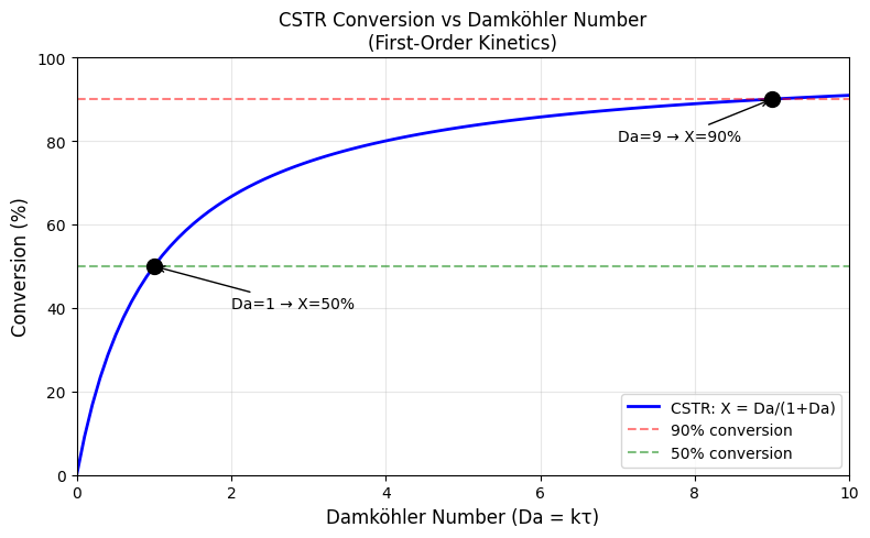
For first-order kinetics in a CSTR:
The Damköhler number \(Da = k\tau\) characterizes the system:
\(Da \ll 1\): Reaction is slow compared to residence time → low conversion
\(Da \gg 1\): Reaction is fast compared to residence time → high conversion
# Setup
import jax.numpy as jnp
import jax
jax.config.update("jax_enable_x64", True)
import matplotlib.pyplot as plt
import numpy as np
# Visualize conversion vs Damköhler number

Da = np.linspace(0, 10, 100)
X_cstr = Da / (1 + Da)

fig, ax = plt.subplots(figsize=(8, 5))
ax.plot(Da, X_cstr * 100, 'b-', linewidth=2, label='CSTR: X = Da/(1+Da)')
ax.axhline(y=90, color='r', linestyle='--', alpha=0.5, label='90% conversion')
ax.axhline(y=50, color='g', linestyle='--', alpha=0.5, label='50% conversion')

# Mark specific points
ax.plot(1, 50, 'ko', markersize=10)
ax.annotate('Da=1 → X=50%', xy=(1, 50), xytext=(2, 40),
            arrowprops=dict(arrowstyle='->', color='black'),
            fontsize=10)

ax.plot(9, 90, 'ko', markersize=10)
ax.annotate('Da=9 → X=90%', xy=(9, 90), xytext=(7, 80),
            arrowprops=dict(arrowstyle='->', color='black'),
            fontsize=10)

ax.set_xlabel('Damköhler Number (Da = kτ)', fontsize=12)
ax.set_ylabel('Conversion (%)', fontsize=12)
ax.set_title('CSTR Conversion vs Damköhler Number\n(First-Order Kinetics)', fontsize=12)
ax.legend()
ax.grid(True, alpha=0.3)
ax.set_xlim(0, 10)
ax.set_ylim(0, 100)

plt.tight_layout()
Implementation from Scratch#
Let’s implement a CSTR solver step by step.
The Problem Setup#
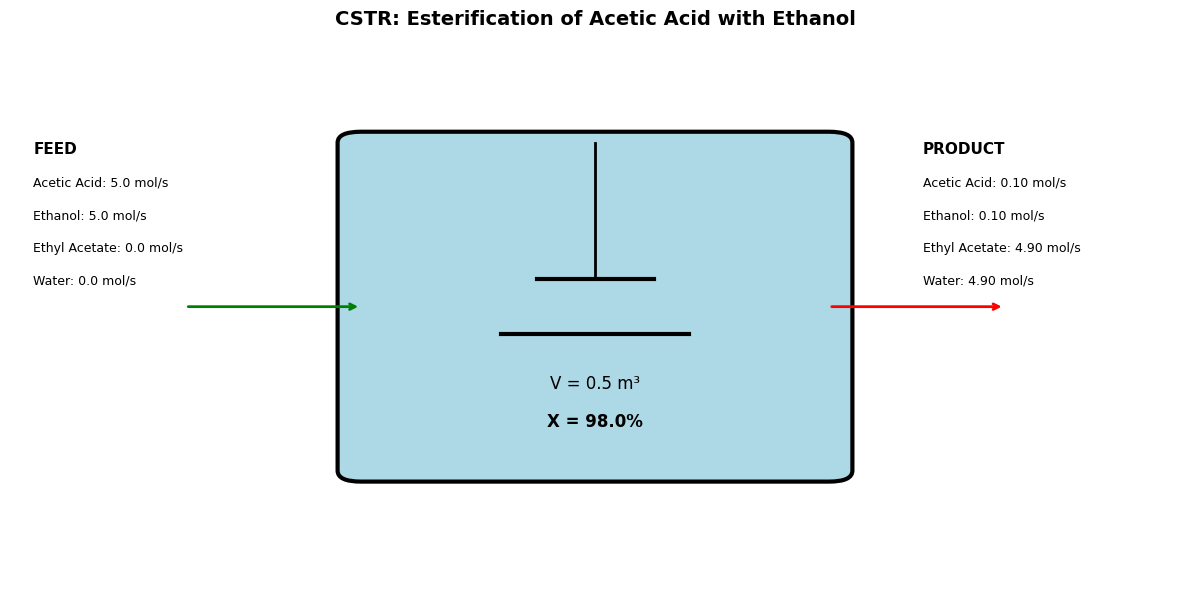
Reaction: Esterification of acetic acid with ethanol
Kinetics: Second-order, \(r = k \cdot C_A \cdot C_B\)
Given:
Feed: 5 mol/s acetic acid, 5 mol/s ethanol, 350 K
Reactor volume: 0.5 m³
Volumetric flow: 0.01 m³/s
Rate constant: k = 0.1 m³/(mol·s) at 350 K
# Step 1: Define the problem parameters

# Feed conditions
F_A_in = 5.0    # Acetic acid, mol/s
F_B_in = 5.0    # Ethanol, mol/s
F_C_in = 0.0    # Ethyl acetate, mol/s
F_D_in = 0.0    # Water, mol/s

# Reactor parameters
V = 0.5         # Reactor volume, m³
Q = 0.01        # Volumetric flow rate, m³/s
tau = V / Q     # Residence time, s

# Kinetics
k = 0.1         # Rate constant, m³/(mol·s)

print("CSTR Problem Setup")
print("=" * 40)
print(f"Feed: F_A = {F_A_in} mol/s, F_B = {F_B_in} mol/s")
print(f"Reactor volume: V = {V} m³")
print(f"Volumetric flow: Q = {Q} m³/s")
print(f"Residence time: τ = V/Q = {tau} s")
print(f"Rate constant: k = {k} m³/(mol·s)")
CSTR Problem Setup
========================================
Feed: F_A = 5.0 mol/s, F_B = 5.0 mol/s
Reactor volume: V = 0.5 m³
Volumetric flow: Q = 0.01 m³/s
Residence time: τ = V/Q = 50.0 s
Rate constant: k = 0.1 m³/(mol·s)
# Step 2: Write the rate expression

def reaction_rate(C_A, C_B, k):
    """
    Rate of reaction A + B -> C + D

    r = k * C_A * C_B  (second-order)

    Returns:
        r: Reaction rate in mol/(m³·s)
    """
    return k * C_A * C_B

# Test with inlet concentrations
C_A_in = F_A_in / Q
C_B_in = F_B_in / Q
r_inlet = reaction_rate(C_A_in, C_B_in, k)

print(f"Inlet concentrations:")
print(f"  C_A = {C_A_in} mol/m³")
print(f"  C_B = {C_B_in} mol/m³")
print(f"Reaction rate at inlet conditions: r = {r_inlet} mol/(m³·s)")
Inlet concentrations:
  C_A = 500.0 mol/m³
  C_B = 500.0 mol/m³
Reaction rate at inlet conditions: r = 25000.0 mol/(m³·s)
# Step 3: Write the CSTR equations
#
# For each species:
# F_i_out = F_i_in + V * r_i
#
# Stoichiometry: A + B -> C + D
# r_A = -r (consumed)
# r_B = -r (consumed)
# r_C = +r (produced)
# r_D = +r (produced)

def cstr_equations_raw(F_out, F_in, V, Q, k):
    """
    CSTR equations for A + B -> C + D.

    Given outlet flows F_out, compute the residuals (should be zero at solution).

    Args:
        F_out: [F_A_out, F_B_out, F_C_out, F_D_out] (the unknowns)
        F_in: [F_A_in, F_B_in, F_C_in, F_D_in] (given)
        V: Reactor volume
        Q: Volumetric flow rate
        k: Rate constant

    Returns:
        Residuals: F_out - F_in - V*r_i (should be zero)
    """
    F_A_out, F_B_out, F_C_out, F_D_out = F_out
    F_A_in, F_B_in, F_C_in, F_D_in = F_in

    # Concentrations (from OUTLET, due to perfect mixing)
    C_A = F_A_out / Q
    C_B = F_B_out / Q

    # Reaction rate (at outlet conditions!)
    r = reaction_rate(C_A, C_B, k)

    # CSTR equations: F_out = F_in + V * r_i
    # Rearranged to residual form: F_out - F_in - V*r_i = 0
    residual_A = F_A_out - F_A_in - V * (-r)  # A consumed
    residual_B = F_B_out - F_B_in - V * (-r)  # B consumed
    residual_C = F_C_out - F_C_in - V * (+r)  # C produced
    residual_D = F_D_out - F_D_in - V * (+r)  # D produced

    return jnp.array([residual_A, residual_B, residual_C, residual_D])

print("CSTR equations defined.")
print("These are 4 nonlinear equations in 4 unknowns (F_A_out, F_B_out, F_C_out, F_D_out).")
CSTR equations defined.
These are 4 nonlinear equations in 4 unknowns (F_A_out, F_B_out, F_C_out, F_D_out).
# Step 4: Solve the equations using optimistix with JAX's automatic Jacobian
# optimistix handles this for us, using JAX autodiff for the Jacobian

import optimistix as optx

def solve_cstr_optimistix(F_in, V, Q, k):
    """
    Solve CSTR equations using optimistix Newton solver.

    The Jacobian is computed automatically by JAX.

    Returns:
        F_out: Converged outlet flows
    """
    # Define the residual function for root finding
    def residual(F_out, args):
        return cstr_equations_raw(F_out, F_in, V, Q, k)

    # Initial guess: assume outlet = inlet (no conversion)
    F_out_guess = jnp.array(F_in)

    # Create Newton solver - JAX computes the Jacobian automatically!
    solver = optx.Newton(rtol=1e-10, atol=1e-10)

    # Solve the root-finding problem: find F_out where residual(F_out) = 0
    solution = optx.root_find(
        residual,
        solver,
        F_out_guess,
        args=None,
        max_steps=50,
        throw=False,
    )

    return solution.value

# Solve
F_in = jnp.array([F_A_in, F_B_in, F_C_in, F_D_in])
F_out_solution = solve_cstr_optimistix(F_in, V, Q, k)

print("Newton-Raphson via optimistix (JAX autodiff Jacobian)")
print("-" * 60)
print(f"Converged outlet flows:")
print(f"  F_A_out = {float(F_out_solution[0]):.4f} mol/s")
print(f"  F_B_out = {float(F_out_solution[1]):.4f} mol/s")
print(f"  F_C_out = {float(F_out_solution[2]):.4f} mol/s")
print(f"  F_D_out = {float(F_out_solution[3]):.4f} mol/s")
WARNING:2026-01-10 21:08:26,553:jax._src.xla_bridge:852: An NVIDIA GPU may be present on this machine, but a CUDA-enabled jaxlib is not installed. Falling back to cpu.
Newton-Raphson via optimistix (JAX autodiff Jacobian)
------------------------------------------------------------
Converged outlet flows:
  F_A_out = 0.0990 mol/s
  F_B_out = 0.0990 mol/s
  F_C_out = 4.9010 mol/s
  F_D_out = 4.9010 mol/s
# Step 5: Analyze the results

F_A_out, F_B_out, F_C_out, F_D_out = F_out_solution

# Conversion
X_A = (F_A_in - float(F_A_out)) / F_A_in
X_B = (F_B_in - float(F_B_out)) / F_B_in

print("\nCSTR Solution (From Scratch)")
print("=" * 50)
print(f"{'Species':<15} {'Inlet (mol/s)':<15} {'Outlet (mol/s)':<15}")
print("-" * 50)
print(f"{'Acetic Acid':<15} {F_A_in:<15.4f} {float(F_A_out):<15.4f}")
print(f"{'Ethanol':<15} {F_B_in:<15.4f} {float(F_B_out):<15.4f}")
print(f"{'Ethyl Acetate':<15} {F_C_in:<15.4f} {float(F_C_out):<15.4f}")
print(f"{'Water':<15} {F_D_in:<15.4f} {float(F_D_out):<15.4f}")
print("-" * 50)
print(f"Total moles: {F_A_in + F_B_in:.4f} → {float(F_A_out + F_B_out + F_C_out + F_D_out):.4f}")
print(f"")
print(f"Conversion of Acetic Acid: X_A = {X_A*100:.2f}%")
print(f"Conversion of Ethanol: X_B = {X_B*100:.2f}%")

# Verify mass balance
print(f"")
print(f"Verification:")
print(f"  Moles A consumed = {F_A_in - float(F_A_out):.4f}")
print(f"  Moles C produced = {float(F_C_out):.4f}")
print(f"  (Should be equal by stoichiometry) ✓" if abs(F_A_in - float(F_A_out) - float(F_C_out)) < 1e-6 else "  ERROR!")
CSTR Solution (From Scratch)
==================================================
Species         Inlet (mol/s)   Outlet (mol/s)
--------------------------------------------------
Acetic Acid     5.0000          0.0990
Ethanol         5.0000          0.0990
Ethyl Acetate   0.0000          4.9010
Water           0.0000          4.9010
--------------------------------------------------
Total moles: 10.0000 → 10.0000

Conversion of Acetic Acid: X_A = 98.02%
Conversion of Ethanol: X_B = 98.02%

Verification:
  Moles A consumed = 4.9010
  Moles C produced = 4.9010
  (Should be equal by stoichiometry) ✓
Using difflow#
Now let’s solve the same problem using difflow. This shows:
The equation: what we derived
Raw code: what we implemented
difflow: the library’s clean interface
from difflow import CSTR, CSTRParams, make_stream, get_flows, IdealThermo, SpeciesData

# Define species (minimal properties for isothermal operation)
species_data = {
    'AceticAcid': SpeciesData(
        name='AceticAcid', MW=60.0,
        Cp_coeffs=(124.0, 0, 0, 0),
        Hvap_coeffs=(23700.0, 0.38, 591.0),
        antoine_coeffs=(10.2, 1936.0, -44.0),
    ),
    'Ethanol': SpeciesData(
        name='Ethanol', MW=46.0,
        Cp_coeffs=(112.0, 0, 0, 0),
        Hvap_coeffs=(38600.0, 0.38, 514.0),
        antoine_coeffs=(10.3, 1593.0, -47.0),
    ),
    'EthylAcetate': SpeciesData(
        name='EthylAcetate', MW=88.0,
        Cp_coeffs=(170.0, 0, 0, 0),
        Hvap_coeffs=(31940.0, 0.38, 523.0),
        antoine_coeffs=(10.1, 1531.0, -51.0),
    ),
    'Water': SpeciesData(
        name='Water', MW=18.0,
        Cp_coeffs=(75.3, 0, 0, 0),
        Hvap_coeffs=(40650.0, 0.38, 647.0),
        antoine_coeffs=(10.2, 1731.0, -40.0),
    ),
}
thermo = IdealThermo(species_data)
species_order = ['AceticAcid', 'Ethanol', 'EthylAcetate', 'Water']
# Define the rate function for difflow

def esterification_rate(C, T, params):
    """
    Rate of A + B -> C + D

    Args:
        C: Dict of concentrations {'AceticAcid': C_A, 'Ethanol': C_B, ...}
        T: Temperature (K)
        params: {'k': rate constant}

    Returns:
        Array of reaction rates [r1]
    """
    k = params['k']
    r = k * C['AceticAcid'] * C['Ethanol']
    return jnp.array([r])

# Stoichiometry matrix: A + B -> C + D
# Rows: species (AceticAcid, Ethanol, EthylAcetate, Water)
# Columns: reactions (just one)
stoich = jnp.array([
    [-1.0],  # AceticAcid consumed
    [-1.0],  # Ethanol consumed
    [+1.0],  # EthylAcetate produced
    [+1.0],  # Water produced
])

print("Stoichiometry matrix:")
print(stoich)
Stoichiometry matrix:
[[-1.]
 [-1.]
 [ 1.]
 [ 1.]]
# Create the CSTR with difflow

cstr_params = CSTRParams(
    V=jnp.array(V),
    rate_fn=esterification_rate,
    stoich=stoich,
    rate_params={'k': jnp.array(k)},
    species_order=species_order,
)

cstr = CSTR(cstr_params, thermo=thermo, mode='isothermal')

# Create inlet stream
inlet = make_stream(
    flows={'AceticAcid': F_A_in, 'Ethanol': F_B_in, 'EthylAcetate': F_C_in, 'Water': F_D_in},
    T=350.0,
    P=101325.0,
)

# Solve
outlet, info = cstr(inlet, T_spec=350.0, volumetric_flow=Q)

print("CSTR Solution (difflow)")
print("=" * 50)
flows_out = get_flows(outlet)
print(f"{'Species':<15} {'Inlet (mol/s)':<15} {'Outlet (mol/s)':<15}")
print("-" * 50)
print(f"{'Acetic Acid':<15} {F_A_in:<15.4f} {float(flows_out['AceticAcid']):<15.4f}")
print(f"{'Ethanol':<15} {F_B_in:<15.4f} {float(flows_out['Ethanol']):<15.4f}")
print(f"{'Ethyl Acetate':<15} {F_C_in:<15.4f} {float(flows_out['EthylAcetate']):<15.4f}")
print(f"{'Water':<15} {F_D_in:<15.4f} {float(flows_out['Water']):<15.4f}")
print("-" * 50)
print(f"")
print(f"Conversion of Acetic Acid: X = {float(info['conversion']['AceticAcid'])*100:.2f}%")
CSTR Solution (difflow)
==================================================
Species         Inlet (mol/s)   Outlet (mol/s)
--------------------------------------------------
Acetic Acid     5.0000          0.0990
Ethanol         5.0000          0.0990
Ethyl Acetate   0.0000          4.9010
Water           0.0000          4.9010
--------------------------------------------------

Conversion of Acetic Acid: X = 98.02%
# Compare raw implementation vs difflow

print("Comparison: Raw Implementation vs difflow")
print("=" * 50)
print(f"{'Species':<15} {'Raw (mol/s)':<15} {'difflow (mol/s)':<15} {'Difference':<15}")
print("-" * 60)

raw_values = [float(F_A_out), float(F_B_out), float(F_C_out), float(F_D_out)]
difflow_values = [float(flows_out['AceticAcid']), float(flows_out['Ethanol']),
                  float(flows_out['EthylAcetate']), float(flows_out['Water'])]
species_names = ['Acetic Acid', 'Ethanol', 'Ethyl Acetate', 'Water']

for name, raw, difflow_val in zip(species_names, raw_values, difflow_values):
    diff = abs(raw - difflow_val)
    print(f"{name:<15} {raw:<15.4f} {difflow_val:<15.4f} {diff:<15.2e}")

print("\n✓ Results match!")
Comparison: Raw Implementation vs difflow
==================================================
Species         Raw (mol/s)     difflow (mol/s) Difference
------------------------------------------------------------
Acetic Acid     0.0990          0.0990          3.75e-16
Ethanol         0.0990          0.0990          3.47e-16
Ethyl Acetate   4.9010          4.9010          0.00e+00
Water           4.9010          4.9010          0.00e+00

✓ Results match!
Visualizing the CSTR#
import matplotlib.pyplot as plt
import matplotlib.patches as patches

def draw_cstr_diagram(inlet_flows, outlet_flows, V, conversion):
    fig, ax = plt.subplots(figsize=(12, 6))

    # CSTR vessel
    vessel = patches.FancyBboxPatch(
        (0.3, 0.2), 0.4, 0.6,
        boxstyle="round,pad=0.02",
        facecolor='lightblue',
        edgecolor='black',
        linewidth=3,
    )
    ax.add_patch(vessel)

    # Stirrer
    ax.plot([0.5, 0.5], [0.8, 0.55], 'k-', linewidth=2)
    ax.plot([0.45, 0.55], [0.55, 0.55], 'k-', linewidth=3)
    ax.plot([0.42, 0.58], [0.45, 0.45], 'k-', linewidth=3)

    # Labels inside
    ax.text(0.5, 0.35, f'V = {V} m³', ha='center', fontsize=12)
    ax.text(0.5, 0.28, f'X = {conversion*100:.1f}%', ha='center', fontsize=12, fontweight='bold')

    # Inlet arrow - starts from left and ends at CSTR boundary
    ax.annotate('', xy=(0.3, 0.5), xytext=(0.15, 0.5),
                arrowprops=dict(arrowstyle='->', lw=2, color='green'))

    # Inlet text - positioned above the arrow
    ax.text(0.02, 0.78, 'FEED', fontsize=11, fontweight='bold')
    ax.text(0.02, 0.72, f'Acetic Acid: {inlet_flows[0]:.1f} mol/s', fontsize=9)
    ax.text(0.02, 0.66, f'Ethanol: {inlet_flows[1]:.1f} mol/s', fontsize=9)
    ax.text(0.02, 0.60, f'Ethyl Acetate: {inlet_flows[2]:.1f} mol/s', fontsize=9)
    ax.text(0.02, 0.54, f'Water: {inlet_flows[3]:.1f} mol/s', fontsize=9)

    # Outlet arrow - starts at CSTR boundary and ends at right
    ax.annotate('', xy=(0.85, 0.5), xytext=(0.7, 0.5),
                arrowprops=dict(arrowstyle='->', lw=2, color='red'))

    # Outlet text - positioned above the arrow
    ax.text(0.78, 0.78, 'PRODUCT', fontsize=11, fontweight='bold')
    ax.text(0.78, 0.72, f'Acetic Acid: {outlet_flows[0]:.2f} mol/s', fontsize=9)
    ax.text(0.78, 0.66, f'Ethanol: {outlet_flows[1]:.2f} mol/s', fontsize=9)
    ax.text(0.78, 0.60, f'Ethyl Acetate: {outlet_flows[2]:.2f} mol/s', fontsize=9)
    ax.text(0.78, 0.54, f'Water: {outlet_flows[3]:.2f} mol/s', fontsize=9)

    ax.set_xlim(0, 1)
    ax.set_ylim(0, 1)
    ax.axis('off')
    ax.set_title('CSTR: Esterification of Acetic Acid with Ethanol', fontsize=14, fontweight='bold')

    plt.tight_layout()
    return fig

fig = draw_cstr_diagram(
    inlet_flows=[F_A_in, F_B_in, F_C_in, F_D_in],
    outlet_flows=difflow_values,
    V=V,
    conversion=float(info['conversion']['AceticAcid'])
)
Try It Yourself!#
Exercise 1: Effect of Residence Time#
Vary the reactor volume (0.1, 0.5, 1.0, 2.0 m³) and plot conversion vs. residence time.
# Your solution here
volumes = [0.1, 0.5, 1.0, 2.0]
conversions = []

for V_test in volumes:
    # Create CSTR with new volume
    # Solve
    # Store conversion
    pass

# Plot conversion vs residence time
Exercise 2: Different Kinetics#
Modify the rate function for a first-order reaction: A → B with r = k·C_A. Compare the analytical solution with your numerical result.
# Your solution here
Exercise 3: Feed Ratio#
What happens if you feed excess ethanol (10 mol/s instead of 5)? Does conversion of acetic acid increase or decrease? Why?
# Your solution here
End-of-Tutorial Problems#
Problem 1: Derive the Design Equation#
For the reaction 2A → B (second-order in A), derive the CSTR design equation and solve for X in terms of k, τ, and C_A0.
Hint: Start from \(F_{A,out} = F_{A,in} + V \cdot r_A\) with \(r_A = -k C_A^2\).
Your derivation here:
Problem 2: Multiple Reactions#
Consider parallel reactions:
A → B (desired), r₁ = k₁·C_A
A → C (undesired), r₂ = k₂·C_A²
If k₁ = 1 /s and k₂ = 0.1 m³/(mol·s), and C_A0 = 10 mol/m³:
a) At what conversion is selectivity to B maximized in a CSTR? b) Is this better or worse than a PFR? (We’ll compare in the next tutorial)
Your answer:
Problem 3: CSTR Sizing#
You need 80% conversion of A in the reaction A → B with k = 0.2 /s. Feed: 100 mol/s of A, volumetric flow 0.5 m³/s.
What volume CSTR is required?
# Your solution here
# Hint: Use the formula X = kτ/(1+kτ) and solve for τ, then V = τ·Q
Key Takeaways#
CSTR design equation: \(F_{i,out} = F_{i,in} + V \cdot r_i\)
Perfect mixing assumption: Outlet composition = composition inside reactor
Residence time: \(\tau = V/Q\) - how long material stays in the reactor
Damköhler number: \(Da = k\tau\) - ratio of reaction rate to flow rate
Conversion depends on kinetics: First-order gives \(X = Da/(1+Da)\)
Newton-Raphson solves nonlinear equations - JAX autodiff computes the Jacobian
Next Steps#
In the next notebook (00e: Single Unit - Energy Balances), we’ll add:
Non-isothermal operation
Heat of reaction effects
Adiabatic vs. isothermal reactors