
Parameter Estimation with difflow.estimation#
This notebook demonstrates the difflow.estimation module — a structured API for
parameter estimation inspired by pyomo’s parmest, powered by JAX autodiff.
What You’ll Learn#
Experiment objects — packaging experimental data
Estimator.fit() — fitting parameters with exact gradients
Confidence intervals — Fisher information CIs via
jax.hessianDiagnostics — R², RMSE, AIC/BIC, residual analysis
Summary reports — one-line result tables
Why Use difflow.estimation?#
Compared to manual parameter estimation (see notebook 14), this module:
Encapsulates the boilerplate (loss functions, scipy calls, CI computation)
Provides JAX-compiled objectives with exact gradients automatically
Offers a consistent
Experimentdata structureIncludes diagnostics (R², AIC, BIC) and formatted summaries
import jax
import jax.numpy as jnp
import numpy as np
import matplotlib.pyplot as plt

jax.config.update("jax_enable_x64", True)

from difflow.estimation import Estimator, Experiment

print("Setup complete")
WARNING:2026-02-24 07:49:32,094:jax._src.xla_bridge:905: Platform 'mps' is experimental and not all JAX functionality may be correctly supported!
WARNING:2026-02-24 07:49:32,123:jax._src.xla_bridge:905: Platform 'METAL' is experimental and not all JAX functionality may be correctly supported!
WARNING: All log messages before absl::InitializeLog() is called are written to STDERR
W0000 00:00:1771937372.124257 20956375 mps_client.cc:510] WARNING: JAX Apple GPU support is experimental and not all JAX functionality is correctly supported!
I0000 00:00:1771937372.130865 20956375 service.cc:145] XLA service 0x822c80b00 initialized for platform METAL (this does not guarantee that XLA will be used). Devices:
I0000 00:00:1771937372.131022 20956375 service.cc:153]   StreamExecutor device (0): Metal, <undefined>
I0000 00:00:1771937372.131992 20956375 mps_client.cc:406] Using Simple allocator.
I0000 00:00:1771937372.132015 20956375 mps_client.cc:384] XLA backend will use up to 55662313472 bytes on device 0 for SimpleAllocator.
Metal device set to: Apple M4 Pro
Setup complete
1. A Simple Linear Model#
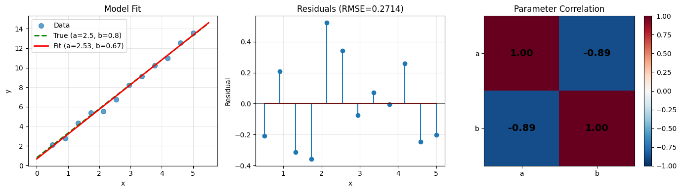
Start with the simplest case: fitting a line \(y = a x + b\) to noisy data.
Step 1: Define the model function#
The model function must follow this convention:
def model_fn(theta_dict, experiment) -> dict[str, float]
theta_dict: parameter names → values (e.g.,{'a': 2.0, 'b': 1.0})experiment: anExperimentobject (read inputs fromexperiment.inputs)Returns: predictions dict with keys matching
experiment.observed
def linear_model(theta, exp):
    """y = a * x + b"""
    return {'y': theta['a'] * exp.inputs['x'] + theta['b']}
Step 2: Create Experiment objects#
Each Experiment holds the inputs, observed outputs, and optional uncertainties.
# True parameters (unknown to the estimator)
a_true, b_true = 2.5, 0.8

# Generate noisy data
rng = np.random.default_rng(42)
x_data = np.linspace(0.5, 5.0, 12)
noise_std = 0.3

experiments = []
for x in x_data:
    y = a_true * x + b_true + noise_std * rng.standard_normal()
    experiments.append(Experiment(
        inputs={'x': float(x)},
        observed={'y': float(y)},
    ))

print(f"Created {len(experiments)} experiments")
print(f"First experiment: {experiments[0]}")
print(f"Output names: {experiments[0].output_names}")
Created 12 experiments
First experiment: Experiment(inputs={'x': 0.5}, observed={'y': 2.141415123926329}, uncertainties=None, name='', metadata={})
Output names: ['y']
Step 3: Create an Estimator and fit#
est = Estimator(linear_model, param_names=['a', 'b'])

result = est.fit(experiments, theta_init={'a': 1.0, 'b': 0.0})

print(f"Converged: {result.converged}")
print(f"Estimated a = {result.theta_opt['a']:.4f} (true: {a_true})")
print(f"Estimated b = {result.theta_opt['b']:.4f} (true: {b_true})")
print(f"Objective (SSE) = {result.objective_value:.6f}")
Converged: True
Estimated a = 2.5328 (true: 2.5)
Estimated b = 0.6673 (true: 0.8)
Objective (SSE) = 0.883816
Step 4: Confidence intervals and diagnostics#
ci = est.confidence_intervals(result, experiments)

print("95% Confidence Intervals:")
for name in ['a', 'b']:
    print(f"  {name}: [{ci.ci_lower[name]:.4f}, {ci.ci_upper[name]:.4f}]  "
          f"(std err = {ci.std_errors[name]:.4f})")

# Check if true values fall within CIs
for name, true_val in [('a', a_true), ('b', b_true)]:
    in_ci = ci.ci_lower[name] <= true_val <= ci.ci_upper[name]
    print(f"  True {name}={true_val} within CI: {in_ci}")
95% Confidence Intervals:
  a: [2.4371, 2.6286]  (std err = 0.0430)
  b: [0.3713, 0.9633]  (std err = 0.1328)
  True a=2.5 within CI: True
  True b=0.8 within CI: True
# Full summary report
print(est.summary(result, experiments))
============================================================
Parameter Estimation Summary
============================================================
Converged: True
Objective value: 0.883816
Iterations: 5

Parameters:
  Name                   Value      Std Err     CI Lower     CI Upper
  ---------------------------------------------------------------
  a                    2.53282    0.0429713      2.43708      2.62857
  b                   0.667271     0.132842     0.371281     0.963261

Diagnostics:
  R-squared:     0.994276
  Adj R-squared: 0.993004
  RMSE:          0.271388
  AIC:           -27.3010
  BIC:           -26.3311
  N obs:         12
  N params:      2
============================================================
# Visualize the fit
fig, axes = plt.subplots(1, 3, figsize=(14, 4))

# Data and fit
x_plot = np.linspace(0, 5.5, 100)
y_true = a_true * x_plot + b_true
y_est = result.theta_opt['a'] * x_plot + result.theta_opt['b']

axes[0].scatter([exp.inputs['x'] for exp in experiments],
                [exp.observed['y'] for exp in experiments],
                label='Data', alpha=0.7, s=50)
axes[0].plot(x_plot, y_true, 'g--', label=f'True (a={a_true}, b={b_true})', lw=2)
axes[0].plot(x_plot, y_est, 'r-', label=f'Fit (a={result.theta_opt["a"]:.2f}, b={result.theta_opt["b"]:.2f})', lw=2)
axes[0].set_xlabel('x')
axes[0].set_ylabel('y')
axes[0].set_title('Model Fit')
axes[0].legend()
axes[0].grid(True, alpha=0.3)

# Residuals
diag = est.diagnostics(result, experiments)
residuals = [r['y'] for r in diag.residuals]
axes[1].stem([exp.inputs['x'] for exp in experiments], residuals)
axes[1].axhline(0, color='k', linewidth=0.5)
axes[1].set_xlabel('x')
axes[1].set_ylabel('Residual')
axes[1].set_title(f'Residuals (RMSE={diag.rmse:.4f})')
axes[1].grid(True, alpha=0.3)

# Correlation matrix
im = axes[2].imshow(ci.correlation, cmap='RdBu_r', vmin=-1, vmax=1)
axes[2].set_xticks([0, 1])
axes[2].set_xticklabels(['a', 'b'])
axes[2].set_yticks([0, 1])
axes[2].set_yticklabels(['a', 'b'])
axes[2].set_title('Parameter Correlation')
for i in range(2):
    for j in range(2):
        axes[2].text(j, i, f'{float(ci.correlation[i, j]):.2f}',
                     ha='center', va='center', fontsize=14, fontweight='bold')
plt.colorbar(im, ax=axes[2])

plt.tight_layout()
plt.show()
2. Nonlinear Model: Exponential Decay#
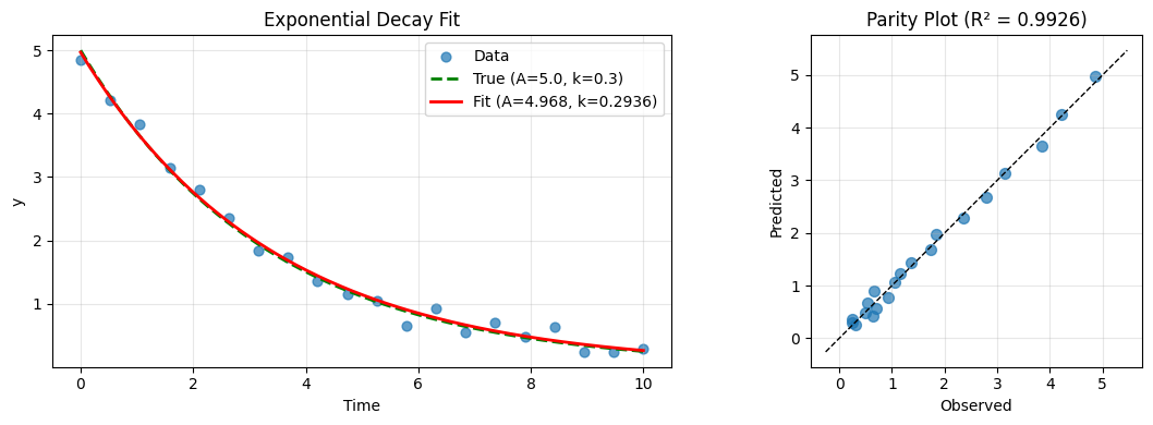
Fit \(y = A \cdot \exp(-k \cdot t)\) — a common kinetic model.
The JAX-powered Hessian gives exact second derivatives for confidence intervals, even for nonlinear models.
def decay_model(theta, exp):
    """y = A * exp(-k * t)"""
    return {'y': theta['A'] * jnp.exp(-theta['k'] * exp.inputs['t'])}

# True parameters
A_true, k_true = 5.0, 0.3

# Generate data
rng = np.random.default_rng(123)
t_data = np.linspace(0.0, 10.0, 20)
decay_experiments = []
for t in t_data:
    y = A_true * np.exp(-k_true * t) + 0.15 * rng.standard_normal()
    decay_experiments.append(Experiment(
        inputs={'t': float(t)},
        observed={'y': float(y)},
    ))

# Fit
est_decay = Estimator(
    decay_model,
    param_names=['A', 'k'],
    param_bounds={'A': (0.1, 20.0), 'k': (0.01, 5.0)},
)
result_decay = est_decay.fit(decay_experiments, theta_init={'A': 3.0, 'k': 0.1})

print(est_decay.summary(result_decay, decay_experiments))
============================================================
Parameter Estimation Summary
============================================================
Converged: True
Objective value: 0.284552
Iterations: 15

Parameters:
  Name                   Value      Std Err     CI Lower     CI Upper
  ---------------------------------------------------------------
  A                    4.96811    0.0609444      4.84007      5.09615
  k                   0.293621   0.00563929     0.281774     0.305469

Diagnostics:
  R-squared:     0.992554
  Adj R-squared: 0.991678
  RMSE:          0.119279
  AIC:           -81.0515
  BIC:           -79.0600
  N obs:         20
  N params:      2
============================================================
# Plot fit and confidence band
ci_decay = est_decay.confidence_intervals(result_decay, decay_experiments)

fig, axes = plt.subplots(1, 2, figsize=(12, 4))

t_plot = np.linspace(0, 10, 200)
y_fit = result_decay.theta_opt['A'] * np.exp(-result_decay.theta_opt['k'] * t_plot)
y_true_plot = A_true * np.exp(-k_true * t_plot)

axes[0].scatter([e.inputs['t'] for e in decay_experiments],
                [e.observed['y'] for e in decay_experiments],
                label='Data', alpha=0.7, s=40)
axes[0].plot(t_plot, y_true_plot, 'g--', label=f'True (A={A_true}, k={k_true})', lw=2)
axes[0].plot(t_plot, y_fit, 'r-', lw=2,
             label=f'Fit (A={result_decay.theta_opt["A"]:.3f}, k={result_decay.theta_opt["k"]:.4f})')
axes[0].set_xlabel('Time')
axes[0].set_ylabel('y')
axes[0].set_title('Exponential Decay Fit')
axes[0].legend()
axes[0].grid(True, alpha=0.3)

# Parity plot
diag_decay = est_decay.diagnostics(result_decay, decay_experiments)
observed = [e.observed['y'] for e in decay_experiments]
predicted = [e.observed['y'] + r['y'] for e, r in zip(decay_experiments, diag_decay.residuals)]
# Actually: predicted = observed + residual, so predicted = observed + (pred - obs) = pred
# Let's compute correctly
predicted = []
for e in decay_experiments:
    p = decay_model(result_decay.theta_opt, e)
    predicted.append(float(p['y']))

axes[1].scatter(observed, predicted, s=50, alpha=0.7)
lims = [min(min(observed), min(predicted)) - 0.5, max(max(observed), max(predicted)) + 0.5]
axes[1].plot(lims, lims, 'k--', lw=1)
axes[1].set_xlabel('Observed')
axes[1].set_ylabel('Predicted')
axes[1].set_title(f'Parity Plot (R² = {diag_decay.r_squared:.4f})')
axes[1].set_aspect('equal')
axes[1].grid(True, alpha=0.3)

plt.tight_layout()
plt.show()
3. Multi-Output Estimation#
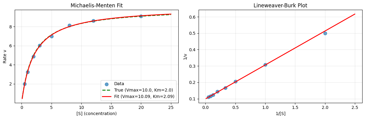
Estimate parameters from models that predict multiple outputs simultaneously. Here we fit a Michaelis-Menten model: \(v = V_{max} \cdot S / (K_m + S)\) and predict both the rate and the substrate consumption.
def mm_model(theta, exp):
    """Michaelis-Menten kinetics with two outputs."""
    S = exp.inputs['S']
    v = theta['Vmax'] * S / (theta['Km'] + S)
    # After time dt, substrate consumed
    dt = exp.inputs['dt']
    S_final = S - v * dt
    return {'rate': v, 'S_final': S_final}

# True parameters
Vmax_true, Km_true = 10.0, 2.0

# Generate data at different substrate concentrations
rng = np.random.default_rng(7)
dt = 0.1
mm_experiments = []
for S in [0.5, 1.0, 2.0, 3.0, 5.0, 8.0, 12.0, 20.0]:
    v_true = Vmax_true * S / (Km_true + S)
    S_final_true = S - v_true * dt
    mm_experiments.append(Experiment(
        inputs={'S': float(S), 'dt': dt},
        observed={
            'rate': float(v_true + 0.3 * rng.standard_normal()),
            'S_final': float(S_final_true + 0.05 * rng.standard_normal()),
        },
    ))

est_mm = Estimator(mm_model, param_names=['Vmax', 'Km'],
                    param_bounds={'Vmax': (0.1, 100.0), 'Km': (0.01, 50.0)})
result_mm = est_mm.fit(mm_experiments, {'Vmax': 5.0, 'Km': 1.0})

print(est_mm.summary(result_mm, mm_experiments))
============================================================
Parameter Estimation Summary
============================================================
Converged: True
Objective value: 0.0666396
Iterations: 11

Parameters:
  Name                   Value      Std Err     CI Lower     CI Upper
  ---------------------------------------------------------------
  Vmax                 10.0908    0.0483005       9.9872      10.1944
  Km                   2.08909    0.0344407      2.01522      2.16295

Diagnostics:
  R-squared:     0.999806
  Adj R-squared: 0.999776
  RMSE:          0.0645366
  AIC:           -83.6967
  BIC:           -82.1515
  N obs:         16
  N params:      2
============================================================
# Visualize Michaelis-Menten fit
fig, axes = plt.subplots(1, 2, figsize=(12, 4))

S_plot = np.linspace(0.1, 25, 200)
v_true_plot = Vmax_true * S_plot / (Km_true + S_plot)
v_fit_plot = result_mm.theta_opt['Vmax'] * S_plot / (result_mm.theta_opt['Km'] + S_plot)

axes[0].scatter([e.inputs['S'] for e in mm_experiments],
                [e.observed['rate'] for e in mm_experiments],
                label='Data', s=60, alpha=0.7)
axes[0].plot(S_plot, v_true_plot, 'g--', lw=2, label=f'True (Vmax={Vmax_true}, Km={Km_true})')
axes[0].plot(S_plot, v_fit_plot, 'r-', lw=2,
             label=f'Fit (Vmax={result_mm.theta_opt["Vmax"]:.2f}, Km={result_mm.theta_opt["Km"]:.2f})')
axes[0].set_xlabel('[S] (concentration)')
axes[0].set_ylabel('Rate v')
axes[0].set_title('Michaelis-Menten Fit')
axes[0].legend()
axes[0].grid(True, alpha=0.3)

# Lineweaver-Burk plot (1/v vs 1/S)
S_data = np.array([e.inputs['S'] for e in mm_experiments])
v_data = np.array([e.observed['rate'] for e in mm_experiments])
axes[1].scatter(1/S_data, 1/v_data, s=60, alpha=0.7)
S_inv = np.linspace(0.01, 1/0.4, 100)
v_inv_fit = (result_mm.theta_opt['Km'] / result_mm.theta_opt['Vmax']) * S_inv + 1/result_mm.theta_opt['Vmax']
axes[1].plot(S_inv, v_inv_fit, 'r-', lw=2)
axes[1].set_xlabel('1/[S]')
axes[1].set_ylabel('1/v')
axes[1].set_title('Lineweaver-Burk Plot')
axes[1].grid(True, alpha=0.3)

plt.tight_layout()
plt.show()
4. Weighted Least Squares#
When measurements have different uncertainties, use weighted SSE. Experiments with smaller uncertainties get more weight in the fit.
# Create experiments with varying measurement uncertainty
rng = np.random.default_rng(99)
weighted_experiments = []

for x in np.linspace(0.5, 5.0, 10):
    # Uncertainty grows with x (e.g., harder to measure at extremes)
    sigma = 0.1 + 0.15 * x
    y = a_true * x + b_true + sigma * rng.standard_normal()
    weighted_experiments.append(Experiment(
        inputs={'x': float(x)},
        observed={'y': float(y)},
        uncertainties={'y': float(sigma)},
    ))

# Compare SSE vs WSSE
est_w = Estimator(linear_model, ['a', 'b'])
result_sse = est_w.fit(weighted_experiments, {'a': 1.0, 'b': 0.0}, objective='sse')
result_wsse = est_w.fit(weighted_experiments, {'a': 1.0, 'b': 0.0}, objective='wsse')

print(f"{'':>15} {'a':>10} {'b':>10}")
print(f"{'True':>15} {a_true:>10.4f} {b_true:>10.4f}")
print(f"{'SSE fit':>15} {result_sse.theta_opt['a']:>10.4f} {result_sse.theta_opt['b']:>10.4f}")
print(f"{'WSSE fit':>15} {result_wsse.theta_opt['a']:>10.4f} {result_wsse.theta_opt['b']:>10.4f}")
print()
print("WSSE gives more weight to precise measurements (low x),")
print("often recovering the true parameters more accurately.")
                         a          b
           True     2.5000     0.8000
        SSE fit     2.5005     0.7545
       WSSE fit     2.4827     0.7992

WSSE gives more weight to precise measurements (low x),
often recovering the true parameters more accurately.
5. CSTR Kinetic Parameter Estimation#
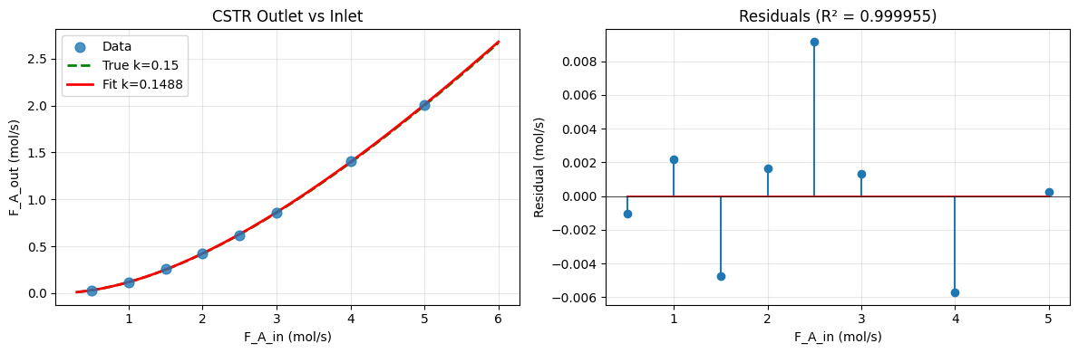
Now let’s use the estimation module with a difflow CSTR model.
We estimate the rate constant k from outlet concentration data at different flow rates.
from difflow import CSTR, CSTRParams, make_stream

# Rate function: A -> B, r = k * C_A
def rate_fn(C, T, params):
    return jnp.array([params['k'] * C['A']])

stoich = jnp.array([[-1.0], [+1.0]])

# True rate constant
k_true_cstr = 0.15

# Generate synthetic CSTR data at different flow rates
rng = np.random.default_rng(0)
flow_rates = [0.5, 1.0, 1.5, 2.0, 2.5, 3.0, 4.0, 5.0]
cstr_experiments = []

for F_A_in in flow_rates:
    cstr = CSTR(
        CSTRParams(V=1.0, rate_fn=rate_fn, stoich=stoich,
                   rate_params={'k': k_true_cstr}, species_order=['A', 'B']),
        mode='isothermal',
    )
    inlet = make_stream({'A': F_A_in, 'B': 0.0}, T=350.0, P=101325.0)
    outlet, _ = cstr(inlet, T_spec=350.0)

    # Add measurement noise
    F_A_out_noisy = float(outlet['F_A']) + 0.01 * rng.standard_normal()
    cstr_experiments.append(Experiment(
        inputs={'F_A_in': F_A_in},
        observed={'F_A_out': F_A_out_noisy},
        name=f'F_A_in={F_A_in}',
    ))

print(f"Created {len(cstr_experiments)} CSTR experiments")
for e in cstr_experiments:
    print(f"  F_A_in={e.inputs['F_A_in']:.1f}  F_A_out={e.observed['F_A_out']:.4f}")
Created 8 CSTR experiments
  F_A_in=0.5  F_A_out=0.0325
  F_A_in=1.0  F_A_out=0.1163
  F_A_in=1.5  F_A_out=0.2564
  F_A_in=2.0  F_A_out=0.4221
  F_A_in=2.5  F_A_out=0.6196
  F_A_in=3.0  F_A_out=0.8608
  F_A_in=4.0  F_A_out=1.4043
  F_A_in=5.0  F_A_out=2.0095
# Model function that wraps the CSTR
def cstr_model(theta, exp):
    """Predict outlet flow from CSTR."""
    cstr = CSTR(
        CSTRParams(V=1.0, rate_fn=rate_fn, stoich=stoich,
                   rate_params={'k': theta['k']}, species_order=['A', 'B']),
        mode='isothermal',
    )
    inlet = make_stream({'A': exp.inputs['F_A_in'], 'B': 0.0}, T=350.0, P=101325.0)
    outlet, _ = cstr(inlet, T_spec=350.0)
    return {'F_A_out': outlet['F_A']}

# Fit
est_cstr = Estimator(cstr_model, ['k'], param_bounds={'k': (0.001, 10.0)})
result_cstr = est_cstr.fit(cstr_experiments, theta_init={'k': 0.05})

print(est_cstr.summary(result_cstr, cstr_experiments))
============================================================
Parameter Estimation Summary
============================================================
Converged: True
Objective value: 0.000148748
Iterations: 5

Parameters:
  Name                   Value      Std Err     CI Lower     CI Upper
  ---------------------------------------------------------------
  k                   0.148792  0.000278216     0.148134      0.14945

Diagnostics:
  R-squared:     0.999955
  Adj R-squared: 0.999947
  RMSE:          0.00431202
  AIC:           -85.1416
  BIC:           -85.0621
  N obs:         8
  N params:      1
============================================================
# Visualize CSTR fit
fig, axes = plt.subplots(1, 2, figsize=(12, 4))

# Outlet flow vs inlet flow
F_in_plot = np.linspace(0.3, 6.0, 50)
F_out_true = []
F_out_fit = []
for F in F_in_plot:
    for k_val, out_list in [(k_true_cstr, F_out_true), (result_cstr.theta_opt['k'], F_out_fit)]:
        cstr = CSTR(
            CSTRParams(V=1.0, rate_fn=rate_fn, stoich=stoich,
                       rate_params={'k': k_val}, species_order=['A', 'B']),
            mode='isothermal',
        )
        inlet = make_stream({'A': float(F), 'B': 0.0}, T=350.0, P=101325.0)
        outlet, _ = cstr(inlet, T_spec=350.0)
        out_list.append(float(outlet['F_A']))

axes[0].scatter([e.inputs['F_A_in'] for e in cstr_experiments],
                [e.observed['F_A_out'] for e in cstr_experiments],
                label='Data', s=60, alpha=0.8, zorder=5)
axes[0].plot(F_in_plot, F_out_true, 'g--', lw=2, label=f'True k={k_true_cstr}')
axes[0].plot(F_in_plot, F_out_fit, 'r-', lw=2,
             label=f'Fit k={result_cstr.theta_opt["k"]:.4f}')
axes[0].set_xlabel('F_A_in (mol/s)')
axes[0].set_ylabel('F_A_out (mol/s)')
axes[0].set_title('CSTR Outlet vs Inlet')
axes[0].legend()
axes[0].grid(True, alpha=0.3)

# Residuals
diag_cstr = est_cstr.diagnostics(result_cstr, cstr_experiments)
resid = [r['F_A_out'] for r in diag_cstr.residuals]
axes[1].stem([e.inputs['F_A_in'] for e in cstr_experiments], resid)
axes[1].axhline(0, color='k', linewidth=0.5)
axes[1].set_xlabel('F_A_in (mol/s)')
axes[1].set_ylabel('Residual (mol/s)')
axes[1].set_title(f'Residuals (R² = {diag_cstr.r_squared:.6f})')
axes[1].grid(True, alpha=0.3)

plt.tight_layout()
plt.show()
6. Comparing Objectives: SSE vs NLL#
The negative_log_likelihood objective assumes Gaussian errors and accounts
for different measurement uncertainties per data point.
# Create experiments with known heteroscedastic noise
rng = np.random.default_rng(77)
nll_experiments = []

for t in np.linspace(0.5, 8.0, 15):
    sigma = 0.05 + 0.03 * t  # Noise grows with t
    y = A_true * np.exp(-k_true * t) + sigma * rng.standard_normal()
    nll_experiments.append(Experiment(
        inputs={'t': float(t)},
        observed={'y': float(y)},
        uncertainties={'y': float(sigma)},
    ))

est_nll = Estimator(decay_model, ['A', 'k'],
                     param_bounds={'A': (0.1, 20.0), 'k': (0.01, 5.0)})

result_sse_nll = est_nll.fit(nll_experiments, {'A': 3.0, 'k': 0.1}, objective='sse')
result_nll = est_nll.fit(nll_experiments, {'A': 3.0, 'k': 0.1}, objective='nll')

print(f"{'':>15} {'A':>10} {'k':>10}")
print(f"{'True':>15} {A_true:>10.4f} {k_true:>10.4f}")
print(f"{'SSE fit':>15} {result_sse_nll.theta_opt['A']:>10.4f} {result_sse_nll.theta_opt['k']:>10.4f}")
print(f"{'NLL fit':>15} {result_nll.theta_opt['A']:>10.4f} {result_nll.theta_opt['k']:>10.4f}")
print()
print("NLL properly weights each observation by its known uncertainty,")
print("giving more influence to precise measurements.")
                         A          k
           True     5.0000     0.3000
        SSE fit     5.0832     0.3077
        NLL fit     5.0494     0.3035

NLL properly weights each observation by its known uncertainty,
giving more influence to precise measurements.
Summary#
Key API#
from difflow.estimation import Estimator, Experiment

# 1. Package data as Experiments
exp = Experiment(inputs={...}, observed={...}, uncertainties={...})

# 2. Define model: theta_dict, experiment -> predictions dict
def model(theta, exp): return {'y': theta['a'] * exp.inputs['x']}

# 3. Create estimator and fit
est = Estimator(model, param_names=['a'], param_bounds={'a': (0, 10)})
result = est.fit(experiments, theta_init={'a': 1.0})

# 4. Analyze
ci = est.confidence_intervals(result, experiments)
diag = est.diagnostics(result, experiments)
print(est.summary(result, experiments))
Objective functions#
Objective |
When to use |
|---|---|
|
Default, equal-weight measurements |
|
Measurements with known, different uncertainties |
|
Gaussian errors with known sigma per observation |
Next steps#
See notebook 23 for bootstrap uncertainty quantification and cross-validation.