Shell-and-Tube Design: Kern Shell Side, U Iteration and Cost Minimisation

difflow.shell_and_tube sizes a 1-2N shell-and-tube exchanger. Given the stream data and a duty it

1. assumes U, gets the area from Q = U A F LMTD,

2. builds a geometry (tube count, shell diameter, baffle spacing),

3. computes the tube-side film coefficient (heat_transfer.internal_h, friction from fluids.friction_factor) and the shell-side one by the Kern method, then U from overall_U with fouling,

4. repeats to a fixed point with optimistix.fixed_point, so the whole design is differentiable.

This notebook shows the Kern pieces, the design loop, the rating cross-check with ShellAndTubeHX, gradients of the area with respect to baffle spacing and tube velocity, and a gradient-based cost minimisation with the tube velocity, baffle spacing and number of passes relaxed to continuous values.

What is and is not validated. The classic Kern kerosene-crude worked example (Kern 1950; Coulson & Richardson Vol 6) is not reproduced: its inputs and printed answers could not be reproduced from memory with confidence. Instead each Kern/tube-side equation is checked against a plain-Python hand calculation and the whole loop against an independent re-implementation (tests/test_shell_and_tube.py). The Kern constants (0.36, 0.55; friction 0.576, 0.19), the bundle-diameter constants and the tube tables were recalled from memory and are not verified against the books. All fluid properties, prices and operating hours below are illustrative placeholders, not data.

import jax, jax.numpy as jnp, numpy as np
import matplotlib.pyplot as plt
from scipy.optimize import minimize
jax.config.update("jax_enable_x64", True)

from difflow import ShellAndTubeHX, ShellAndTubeHXParams, make_stream
from difflow import shell_and_tube as st
import difflow.economics as econ

1. The problem

A hot hydrocarbon (shell side, 5 kg/s, 200 C) is cooled to 100 C by a cooler, more viscous hydrocarbon (tubes, 18 kg/s, 30 C). Properties are illustrative constants, passed explicitly (core SpeciesData has no liquid transport properties). Tubes are 19.05 mm OD, 14.83 mm ID on a 1.25 pitch ratio, triangular layout, 4.88 m long (16 ft); fouling 1e-4 m2K/W on each side.

DO, DI = 0.01905, 0.01483
SHELL = dict(rho=780.0, mu=4.0e-4, k=0.13, Cp=2200.0)    # hot fluid (illustrative)
TUBE  = dict(rho=830.0, mu=2.9e-3, k=0.13, Cp=2050.0)    # cold fluid (illustrative)
hot, cold = {"T": 473.0, "m_dot": 5.0}, {"T": 303.0, "m_dot": 18.0}

def params(**kw):
    base = dict(tube_OD=DO, tube_ID=DI,
                rho_hot=SHELL["rho"], mu_hot=SHELL["mu"], k_hot=SHELL["k"], Cp_hot=SHELL["Cp"],
                rho_cold=TUBE["rho"], mu_cold=TUBE["mu"], k_cold=TUBE["k"], Cp_cold=TUBE["Cp"],
                tube_side="cold", tube_length=4.88, R_fi=1e-4, R_fo=1e-4)
    base.update(kw)
    return st.ShellAndTubeDesignParams(**base)

2. The Kern shell side

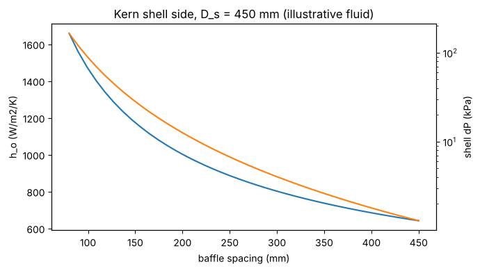
kern_shell_side returns the equivalent diameter D_e, the cross-flow area A_s = (P_t - d_o) D_s l_B / P_t, the mass velocity G_s, Re_s and h_o from Nu = 0.36 Re^0.55 Pr^(1/3) (mu/mu_w)^0.14; kern_shell_pressure_drop adds the shell dP. Closing the baffles raises h_o and raises dP much faster:

Ds, Pt = 0.45, 1.25 * DO
lB = np.linspace(0.08, 0.45, 40)
ho = [float(st.kern_shell_side(5.0, **SHELL, shell_ID=Ds, tube_OD=DO, pitch=Pt, baffle_spacing=b)["h_o"]) for b in lB]
dp = [float(st.kern_shell_pressure_drop(5.0, SHELL["rho"], SHELL["mu"], Ds, DO, Pt, b, 4.88)["dP"]) for b in lB]
r = st.kern_shell_side(5.0, **SHELL, shell_ID=Ds, tube_OD=DO, pitch=Pt, baffle_spacing=0.2)
print({k: round(float(v), 4) for k, v in r.items()})

fig, ax = plt.subplots(figsize=(7, 4))
ax.plot(lB * 1e3, ho, label="h_o (W/m2/K)")
ax.set_xlabel("baffle spacing (mm)"); ax.set_ylabel("h_o (W/m2/K)")
ax2 = ax.twinx(); ax2.semilogy(lB * 1e3, np.array(dp) / 1e3, "C1", label="shell dP (kPa)"); ax2.set_ylabel("shell dP (kPa)")
ax.set_title("Kern shell side, D_s = 450 mm (illustrative fluid)")
plt.tight_layout(); plt.show()

{'De': 0.0135, 'As': 0.018, 'Gs': 277.7778, 'us': 0.3561, 'Re': 9393.3698, 'Pr': 6.7692, 'Nu': 104.2799, 'h_o': 1002.2133}

3. Design by iterating U

ShellAndTubeDesign takes mass flows and one of Q, T_hot_out, T_cold_out. The result holds the geometry, U, area, F, both pressure drops and flags (F < 0.75, dP above its limit, not converged, laminar tubes).

# tube velocity fixed at 1.5 m/s: the tube count follows from the flow, the tube length from the area
design = st.ShellAndTubeDesign(params(tube_length=None, tube_velocity=1.5, dP_tube_max=7e4, dP_shell_max=7e4))
res = design(hot, cold, T_hot_out=373.0)
keys = ["Q", "U", "area", "F", "LMTD", "T_cold_out", "n_tubes", "tube_length", "bundle_ID", "shell_ID",
        "baffle_spacing", "n_baffles", "tube_velocity", "h_i", "h_o", "Re_tube", "Re_shell", "dP_tube", "dP_shell",
        "U_residual"]
for k in keys:
    print(f"{k:>15s} = {float(res[k]):.6g}")
print("converged:", bool(res["converged"]), "| F too low:", bool(res["F_too_low"]),
      "| dP exceeded:", bool(res["dP_tube_exceeded"]), bool(res["dP_shell_exceeded"]))

              Q = 1.1e+06
              U = 391.902
           area = 29.297
              F = 0.947964
           LMTD = 101.065
     T_cold_out = 332.81
        n_tubes = 167.402
    tube_length = 2.92427
      bundle_ID = 0.363977
       shell_ID = 0.413977
 baffle_spacing = 0.165591
      n_baffles = 16.6596
  tube_velocity = 1.5
            h_i = 910.287
            h_o = 1164.09
        Re_tube = 6366.67
       Re_shell = 12332.5
        dP_tube = 21674.4
       dP_shell = 13688.6
     U_residual = 7.76389e-11
converged: True | F too low: False | dP exceeded: False False

The same problem with the tube length fixed at 4.88 m instead (the tube count then follows from the area). The iteration converges to the same U from any typical starting value. The fixed point is not unique with a fixed tube length: more area means more tubes, slower tube flow and a lower h_i, a positive feedback. A very low guess settles on a second, large-area laminar solution, which the result flags (tube_laminar) and warns about; fixing the tube velocity (section 6) removes the feedback.

import warnings
for U0 in (150.0, 500.0, 2000.0, 5000.0, 50.0):
    with warnings.catch_warnings(record=True) as w:
        warnings.simplefilter("always")
        r = st.ShellAndTubeDesign(params(U_guess=U0))(hot, cold, T_hot_out=373.0, warn=True)
    print(f"U_guess {U0:6.0f} -> U = {float(r['U']):8.2f}  A = {float(r['area']):7.2f} m2  Re_tube = {float(r['Re_tube']):8.0f}"
          + ("   <- laminar, large-area branch (warned)" if len(w) else ""))

U_guess    150 -> U =   861.72  A =   13.32 m2  Re_tube =    23362

U_guess    500 -> U =   861.72  A =   13.32 m2  Re_tube =    23362

U_guess   2000 -> U =   861.72  A =   13.32 m2  Re_tube =    23362

U_guess   5000 -> U =   861.72  A =   13.32 m2  Re_tube =    23362

U_guess     50 -> U =    54.39  A =  211.11 m2  Re_tube =     1474   <- laminar, large-area branch (warned)

4. Rating cross-check

ShellAndTubeHX rates a 1-2N exchanger from UA. Fed the design’s U * A it must return the design duty and outlet temperatures. (Doing this check exposed two bugs in the rating path, fixed in the same change: the Bowman F factor ignored its own formula for |R-1| > 0.075, and ShellAndTubeHX computed Q = F Q_cc instead of Q = UA F LMTD. See the changelog.) rate re-rates any given geometry with the correlations.

MW = 0.018      # arbitrary: only C = m Cp matters
hx = ShellAndTubeHX(ShellAndTubeHXParams(UA=float(res["U"] * res["area"]),
                                         Cp_hot=SHELL["Cp"] * MW, Cp_cold=TUBE["Cp"] * MW))
ho_, co_, info = hx(make_stream({"A": 5.0 / MW}, 473.0, 101325.0), make_stream({"A": 18.0 / MW}, 303.0, 101325.0))
print(f"design : Q = {float(res['Q']):.1f} W, T_hot_out = 373.000 K, T_cold_out = {float(res['T_cold_out']):.4f} K, F = {float(res['F']):.5f}")
print(f"rating : Q = {float(info['Q']):.1f} W, T_hot_out = {float(ho_['T']):.3f} K, T_cold_out = {float(co_['T']):.4f} K, F = {float(info['F_correction']):.5f}")
rt = design.rate(hot, cold, res["n_tubes"], res["tube_length"], res["shell_ID"], res["baffle_spacing"])
print(f"rate() : Q = {float(rt['Q']):.1f} W (geometry -> correlations -> effectiveness)")

design : Q = 1100000.0 W, T_hot_out = 373.000 K, T_cold_out = 332.8103 K, F = 0.94796
rating : Q = 1100000.0 W, T_hot_out = 373.000 K, T_cold_out = 332.8103 K, F = 0.94796
rate() : Q = 1100000.0 W (geometry -> correlations -> effectiveness)

5. Gradients through the fixed point

With the tube velocity fixed the tube count follows from the flow and the tube length from the area. The area is then a differentiable function of baffle spacing and tube velocity (implicit-function-theorem gradient of optx.fixed_point):

vd = st.ShellAndTubeDesign(params(tube_length=None, tube_velocity=1.2, baffle_spacing=0.25, tol=1e-13))
area = lambda lB, v: vd(hot, cold, T_hot_out=373.0, baffle_spacing=lB, tube_velocity=v, warn=False)["area"]
g = jax.grad(area, argnums=(0, 1))(0.25, 1.2)
h = 1e-5
fd = ((area(0.25 + h, 1.2) - area(0.25 - h, 1.2)) / (2 * h), (area(0.25, 1.2 + h) - area(0.25, 1.2 - h)) / (2 * h))
print(f"A = {float(area(0.25, 1.2)):.3f} m2")
print(f"dA/dl_B : jax.grad {float(g[0]):+.5f}  finite difference {float(fd[0]):+.5f}  m2 per m")
print(f"dA/dv   : jax.grad {float(g[1]):+.5f}  finite difference {float(fd[1]):+.5f}  m2 per m/s")

A = 36.903 m2
dA/dl_B : jax.grad +28.58865  finite difference +28.58865  m2 per m
dA/dv   : jax.grad -21.68420  finite difference -21.68420  m2 per m/s

6. Gradient-based cost minimisation

Minimise annualised capital (heat_exchanger_cost(area) times a capital charge) plus pumping cost, over the continuous tube velocity, baffle spacing and number of tube passes, subject to dP limits on both sides and Re_tube >= 1e4 (keeps the design out of the unphysical interpolated transition range).

Every price, the annuity factor, the operating hours, the pump efficiency and the dP limits are illustrative placeholders. heat_exchanger_cost is the library’s power-law correlation (11000 + 340 A^0.6, 2019 dollars escalated), not a quote. SLSQP uses jax.grad/jax.jacobian of the design as exact gradients.

ANN, HOURS, PRICE_KWH, ETA, DPMAX = 0.20, 8000.0, 0.10, 0.60, 7.0e4    # all illustrative
design_v = st.ShellAndTubeDesign(params(tube_length=None, tube_velocity=1.0, tol=1e-12, U_guess=800.0))

def solve(x):
    v, lb, npass = jnp.exp(x[0]), jnp.exp(x[1]), x[2]
    return design_v(hot, cold, T_hot_out=373.0, tube_velocity=v, baffle_spacing=lb, n_tube_passes=npass, warn=False)

def cost_terms(r):
    capital = ANN * econ.heat_exchanger_cost(r["area"])
    power = (cold["m_dot"] / TUBE["rho"] * r["dP_tube"] + hot["m_dot"] / SHELL["rho"] * r["dP_shell"]) / ETA   # W
    return capital, power / 1e3 * HOURS * PRICE_KWH

total = lambda x: sum(cost_terms(solve(x)))
cons = lambda x: (lambda r: jnp.array([DPMAX - r["dP_tube"], DPMAX - r["dP_shell"], r["Re_tube"] - 1e4]) / jnp.array([1e4, 1e4, 1e3]))(solve(x))
vg, cj = jax.jit(jax.value_and_grad(total)), jax.jit(jax.jacobian(cons))
cf = jax.jit(cons)

x0 = np.array([np.log(1.0), np.log(0.25), 2.0])
sol = minimize(lambda x: tuple(np.asarray(a) for a in vg(x)), x0, jac=True, method="SLSQP",
               bounds=[(np.log(0.3), np.log(3.0)), (np.log(0.05), np.log(1.0)), (1.0, 8.0)],
               constraints=[{"type": "ineq", "fun": lambda x: np.asarray(cf(x)), "jac": lambda x: np.asarray(cj(x))}])
print(sol.message, "| iterations:", sol.nit)
for name, x in (("start", x0), ("optimum", sol.x)):
    r = solve(x); cap, pump = cost_terms(r)
    print(f"{name:8s} v = {np.exp(x[0]):.3f} m/s  l_B = {np.exp(x[1])*1e3:6.1f} mm  passes = {x[2]:.2f}  "
          f"A = {float(r['area']):6.2f} m2  L = {float(r['tube_length']):.2f} m  Ds = {float(r['shell_ID']):.3f} m  "
          f"dP_t = {float(r['dP_tube'])/1e3:5.1f} kPa  dP_s = {float(r['dP_shell'])/1e3:5.1f} kPa  "
          f"Re_t = {float(r['Re_tube']):.0f}  cost = {float(cap + pump):,.0f} $/yr (capital {float(cap):,.0f} + pumping {float(pump):,.0f})")

Optimization terminated successfully | iterations: 10

start    v = 1.000 m/s  l_B =  250.0 mm  passes = 2.00  A =  42.25 m2  L = 2.81 m  Ds = 0.487 m  dP_t =  10.0 kPa  dP_s =   3.6 kPa  Re_t = 4244  cost = 4,157 $/yr (capital 3,837 + pumping 320)

optimum  v = 2.356 m/s  l_B =  249.8 mm  passes = 1.00  A =  22.91 m2  L = 7.18 m  Ds = 0.258 m  dP_t =  48.6 kPa  dP_s =  15.5 kPa  Re_t = 10000  cost = 5,107 $/yr (capital 3,570 + pumping 1,537)

The starting point violates the Re_tube >= 1e4 constraint (Re about 4200), so its lower cost is not comparable. The optimum sits on the Re_tube = 1e4 constraint with the passes at their lower bound of 1: with the library’s shallow capital correlation (A^0.6 over a fixed term) and these placeholder prices the pumping cost is small, so the economics ask for as much area reduction as the constraints allow. That is a statement about the placeholder economics, not about heat exchangers. A velocity scan at the optimal baffle spacing and passes shows the trade (capital falls, pumping rises) and that the gradient-based optimum is the scan minimum among feasible points:

vs = np.linspace(0.5, 3.0, 40)
xs = [np.array([np.log(v), sol.x[1], sol.x[2]]) for v in vs]
caps, pumps = zip(*[(float(a), float(b)) for a, b in (cost_terms(solve(x)) for x in xs)])
feas = [bool(np.all(np.asarray(cf(x)) >= 0)) for x in xs]
tot = np.array(caps) + np.array(pumps)

fig, ax = plt.subplots(figsize=(7, 4))
ax.plot(vs, caps, label="annualised capital"); ax.plot(vs, pumps, label="pumping")
ax.plot(vs, tot, "k", lw=2, label="total")
ax.plot(vs[~np.array(feas)], tot[~np.array(feas)], "rx", label="violates dP / Re limit")
ax.axvline(np.exp(sol.x[0]), color="g", ls="--", label="gradient-based optimum")
ax.set_xlabel("tube velocity (m/s)"); ax.set_ylabel("$/yr (illustrative)"); ax.legend(fontsize=8); plt.tight_layout(); plt.show()
best = vs[np.argmin(np.where(feas, tot, np.inf))]
print(f"scan minimum among feasible points: v = {best:.2f} m/s; gradient-based optimum v = {np.exp(sol.x[0]):.3f} m/s")

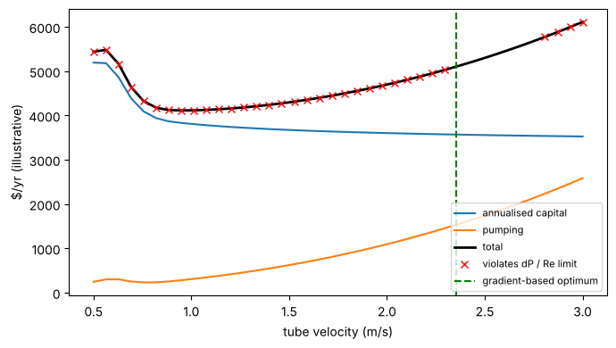
scan minimum among feasible points: v = 2.36 m/s; gradient-based optimum v = 2.356 m/s

Rounding and re-rating

Tube count, passes and baffle count are real numbers in the optimisation. To build the exchanger, round_design rounds the tube count up, the passes to the nearest standard even count, the baffle spacing down and the shell diameter up to a standard step, and rate re-rates that geometry (velocities, h_i, h_o and both dP all change):

opt = solve(sol.x)
g = st.round_design(opt)
print({k: round(v, 4) for k, v in g.items()})
dsg = st.ShellAndTubeDesign(params(tube_length=None, tube_velocity=1.0))
rr = dsg.rate(hot, cold, **g)
print(f"re-rated: Q = {float(rr['Q'])/1e3:.1f} kW (target {float(opt['Q'])/1e3:.1f}), T_hot_out = {float(rr['T_hot_out']):.2f} K, "
      f"area = {float(rr['area']):.2f} m2 (design {float(opt['area']):.2f}), dP_t = {float(rr['dP_tube'])/1e3:.1f} kPa, "
      f"dP_s = {float(rr['dP_shell'])/1e3:.1f} kPa")

{'n_tubes': 54.0, 'n_tube_passes': 1.0, 'tube_length': 7.1825, 'shell_ID': 0.2667, 'baffle_spacing': 0.225}
re-rated: Q = 1113.0 kW (target 1100.0), T_hot_out = 371.82 K, area = 23.21 m2 (design 22.91), dP_t = 47.4 kPa, dP_s = 20.3 kPa

7. Condensing or boiling shell side

A phase-changing side is isothermal (hot_isothermal=True: F = 1) and its film coefficient comes from outside the Kern method: a number, or a function of the geometry such as nusselt_film_condensation for a horizontal tube bank. Shell dP is not modelled in this mode. Steam at 100 C (illustrative properties) condensing on the outside of a tube bundle heating the cold oil:

from difflow import heat_transfer as ht
def shell_h(g):
    n_col = jnp.sqrt(g["n_tubes"])          # tubes per vertical row: a crude placeholder
    return ht.nusselt_film_condensation(k_l=0.68, rho_l=958.0, rho_v=0.6, mu_l=2.8e-4, h_fg=2.257e6,
                                        Cp_l=4216.0, dT=10.0, L=g["tube_OD"], n_tubes=n_col)
cond = st.ShellAndTubeDesign(params(hot_isothermal=True, shell_h=shell_h, tube_length=None, tube_velocity=1.5, R_fo=1e-4))
rc = cond({"T": 373.15, "m_dot": 1.0}, cold, Q=1.0e6)
print(f"h_o = {float(rc['h_o']):.0f} W/m2/K, U = {float(rc['U']):.0f}, A = {float(rc['area']):.2f} m2, "
      f"Nt = {float(rc['n_tubes']):.0f}, T_cold_out = {float(rc['T_cold_out']):.1f} K, F = {float(rc['F'])}")
print("dA/dQ =", float(jax.grad(lambda Q: cond({"T": 373.15, "m_dot": 1.0}, cold, Q=Q, warn=False)["area"])(1.0e6)), "m2/W")

h_o = 7172 W/m2/K, U = 546, A = 33.01 m2, Nt = 167, T_cold_out = 330.1 K, F = 1.0

dA/dQ = 4.2556690612549905e-05 m2/W