
Siting a 100 MW Data Center: an Interconnection Screening Study#
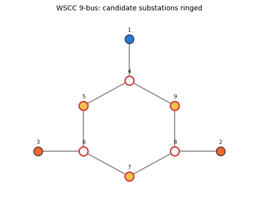
The request. A developer wants to connect a 100 MW data center to the transmission system and has options at six substations. The utility has to answer three questions before it can make an offer:
Where should it connect?
What does it cost the system to serve it there?
What has to be built so that the system still meets its reliability criteria with the new load in place?
The answer is not simply the site with the lowest price. A site can be cheap to serve on a normal day and still leave the system unable to survive the loss of a line or a generating unit. An interconnection study therefore weighs cost against reliability under contingencies and against the network upgrades needed to restore it. This notebook works through that study on the WSCC 9-bus test system, in the stages a planning engineer would follow:
stage |
question |
method |
|---|---|---|
0 |
what is already wrong with the system? |
base-case AC-OPF and N-1 scan |
1 |
which sites look cheapest? |
nodal prices from one AC-OPF |
2 |
what does each site actually cost? |
AC-OPF re-solved with the load at each site |
3 |
does the system survive N-1 at each site? |
line outages (no redispatch) and unit outages (with redispatch) |
4 |
what upgrades would fix the finalists? |
sizing by sensitivity, verified by re-solving |
5 |
how much room is left to grow? |
hosting capacity, without and with N-1 |
6 |
does the answer hold with load growth? |
the same scan at +10 % load |
It ends with a scorecard and a recommendation.
Study basis and assumptions#
Every interconnection study begins by stating its basis, because the answer is only as good as the case it was run on.
item |
assumption |
|---|---|
system |
WSCC 9-bus (MATPOWER |
planning case |
load as published; a +10 % load-growth case as a sensitivity |
new load |
100 MW at 0.98 power factor lagging (20.3 MVAr), constant power: a data center draws near-constant power through its UPS and power supplies |
candidate sites |
the six transmission substations, buses 4 to 9. Buses 1 to 3 are generator terminals; co-locating a load behind a plant’s meter raises separate regulatory and operating questions and is out of scope here |
dispatch |
security-unconstrained AC optimal power flow ( |
thermal limits |
each branch’s single rating in the case file, used as both the normal and the emergency rating |
voltage limits |
0.90 to 1.10 pu, normal and post-contingency |
contingencies |
single outages (N-1) in the spirit of NERC TPL-001 category P1: each of the 6 lines, and each of the 2 non-slack units with the step-up branch that connects it |
post-contingency state, line outage |
AC power flow with the pre-contingency dispatch and generator voltage setpoints held; the slack unit absorbs the change in losses. This is the instantaneous state before operators act |
post-contingency state, unit outage |
AC-OPF re-dispatch of the remaining units: losing a unit is covered by reserves, and the test is whether a dispatch inside every limit exists |
attribution |
a violation counts against the project only if it is new, or an existing one worsened by more than 1 % of rating or 0.01 pu |
What this study does not cover, and a full system impact study would: short-circuit duty, transient and voltage stability, N-1-1 and breaker-failure events, protection, and production-cost simulation over the hours of a year. It is a screening study: its job is to choose where to look closely.
import jax
jax.config.update("jax_enable_x64", True)

from dataclasses import replace

import matplotlib.pyplot as plt
import numpy as np

import difflow_power as dp
from difflow_power.network import Load
from difflow_power.residuals import power_state_layout

PROJECT_MW = 100.0
POWER_FACTOR = 0.98
CANDIDATES = ["4", "5", "6", "7", "8", "9"]
LINES = ["br2", "br3", "br5", "br6", "br8", "br9"]     # the six network lines
UNITS = ["g2", "g3"]                                   # g1 is the slack unit
TOL = 0.01                                             # attribution threshold

case = dp.cases.case9()
print(case.summary())


def label(net, branch):
    br = net.branches[branch]
    return f"{br.from_bus}-{br.to_bus}"


for b in LINES:
    br = case.branches[b]
    print(f"  line {label(case, b):4s} rating {br.rate_mva:5.0f} MVA")
case9 (WSCC 9-bus): 9 buses (1 slack, 2 PV, 6 PQ), 9 branches (0 transformers, 9 rated), 3 generators (820 MW capacity), 3 loads (315.0 MW + 115.0 MVAr), 1 loops, base 100 MVA
  line 4-5  rating   250 MVA
  line 5-6  rating   150 MVA
  line 6-7  rating   150 MVA
  line 7-8  rating   250 MVA
  line 8-9  rating   250 MVA
  line 9-4  rating   250 MVA
POS = {"1": (0.0, 2.1), "4": (0.0, 1.1), "5": (-1.1, 0.5), "9": (1.1, 0.5),
       "6": (-1.1, -0.6), "8": (1.1, -0.6), "7": (0.0, -1.2),
       "3": (-2.2, -0.6), "2": (2.2, -0.6)}
fig, ax = plt.subplots(figsize=(6.5, 5))
dp.draw_network(case, pos=POS, highlight=CANDIDATES, ax=ax,
                title="WSCC 9-bus: candidate substations ringed")
plt.show()
Tools for the study#
Four small functions do all the work. with_load attaches the data center;
contingency_scan runs every N-1 event and returns each limit it breaks, as a
record keyed by (event, element); attributable compares a scan against the
pre-project scan and keeps only what the project caused or worsened.
def with_load(net, bus, mw=PROJECT_MW):
    loads = dict(net.loads)
    loads["dc"] = Load(bus=bus, p_mw=mw,
                       q_mvar=mw * np.tan(np.arccos(POWER_FACTOR)),
                       name="data center")
    return replace(net, loads=loads)


def with_capacitor(net, bus, mvar):
    buses = dict(net.buses)
    buses[bus] = replace(buses[bus], b_shunt_mvar=buses[bus].b_shunt_mvar + mvar)
    return replace(net, buses=buses)


def line_outage_case(net, opf, line):
    # Pre-contingency dispatch and voltage setpoints held; the line removed.
    gens = {g: replace(u, p_mw=opf.pg_mw[g]) for g, u in net.generators.items()}
    buses = {b: replace(x, vm_setpoint=opf.vm[b]) for b, x in net.buses.items()}
    branches = {a: x for a, x in net.branches.items() if a != line}
    return replace(net, branches=branches, generators=gens, buses=buses)


def unit_outage_case(net, unit):
    bus = net.generators[unit].bus
    gens = {g: u for g, u in net.generators.items() if g != unit}
    buses = {b: (replace(x, kind="pq") if b == bus else x)
             for b, x in net.buses.items()}
    return replace(net, generators=gens, buses=buses)


def contingency_scan(net, opf):
    # Returns {(event, element): {"excess": ..., "text": ...}}.
    out = {}
    for line in LINES:
        event = f"loss of line {label(net, line)}"
        post = line_outage_case(net, opf, line)
        pf = dp.solve_power_flow(post)
        if not pf.converged:
            out[(event, "solution")] = dict(
                excess=np.inf, text="no power-flow solution (voltage collapse?)")
            continue
        rep = dp.operating_report(pf.x, post)
        for br, loading in rep.thermal_violations.items():
            out[(event, br)] = dict(
                excess=loading - 1.0,
                text=f"line {label(net, br)} at {100 * loading:.0f} % of rating")
        for bus, dv in rep.voltage_violations.items():
            out[(event, f"bus {bus}")] = dict(
                excess=abs(dv), text=f"bus {bus} at {pf.vm[bus]:.3f} pu")
    for unit in UNITS:
        event = f"loss of unit {unit[1:]}"
        post = unit_outage_case(net, unit)
        res = dp.solve_acopf(post)
        if not (res.converged and dp.operating_report(res.x, post).feasible):
            out[(event, "redispatch")] = dict(
                excess=np.inf, text="no feasible redispatch found")
    return out


def attributable(before, after, tol=TOL):
    return {k: v for k, v in after.items()
            if k not in before or v["excess"] > before[k]["excess"] + tol}


def show(records, indent="  "):
    if not records:
        print(indent + "none")
    for (event, _), r in sorted(records.items()):
        print(f"{indent}{event:22s} {r['text']}")
Stage 0: the system before the project#
Run the base case first. Two things come out of it: the pre-project cost and prices that the screen will use, and the list of N-1 problems that already exist. A study that skipped this step would charge the project for problems it did not cause.
base_opf = dp.solve_acopf(case)
print(base_opf.summary())
base_scan = contingency_scan(case, base_opf)
print("\nN-1 violations that exist BEFORE the project:")
show(base_scan)
case9 (WSCC 9-bus): converged in 19 interior-point iterations, cost $5296.69/h for 315.0 MW load (3.31 MW loss); LMP 24.03 to 25.00 $/MWh; 3 binding constraints (vm_1_max, vm_6_max, vm_8_max)
N-1 violations that exist BEFORE the project:
  loss of line 8-9       bus 9 at 0.896 pu
  loss of line 9-4       bus 9 at 0.791 pu
The test system is not N-1 secure as published. Bus 9 serves 125 MW, the largest load, through two lines. Lose line 9-4 and it hangs on the long 8-9 line alone, dropping to about 0.79 pu; lose 8-9 and it sits just under the 0.90 pu limit. That is an existing deficiency for the utility to fix, not something the data center caused. It is recorded here so the project is not charged with it, and every later scan is compared against this list.
Stage 1: screen every site from one solve#
The nodal price at a bus is the marginal cost of serving load there. Price times 100 MW is therefore a first-order estimate of what the project adds to system cost, and it comes from the base solve already in hand: one solve for all six sites, or for six hundred.
lmp = base_opf.lmp_mw
screen = {b: lmp[b] * PROJECT_MW for b in CANDIDATES}
print(f"{'site':>5} {'LMP $/MWh':>10} {'est. $/h':>9}")
for b in sorted(CANDIDATES, key=screen.get):
    print(f"{'bus ' + b:>5} {lmp[b]:10.2f} {screen[b]:9.0f}")
 site  LMP $/MWh  est. $/h
bus 8      24.03      2403
bus 6      24.08      2408
bus 7      24.25      2425
bus 4      24.76      2476
bus 5      25.00      2500
bus 9      25.00      2500
The prices span only about 4 %, because nothing is congested in the base case: the spread is losses. On cost alone the screen points at buses 8 and 6 and away from 5 and 9.
Stage 2: re-solve with the project at each site#
100 MW is a third of the system load, not a marginal increment, so each site is re-solved with the load in place. The re-solve also reports what the screen cannot: the change in losses, the lowest voltage and the limits that bind.
site_opf = {}
print(f"{'site':>5} {'screen $/h':>10} {'re-solve $/h':>12} {'gap':>6} "
      f"{'d losses MW':>11} {'min V pu':>8}  binding")
for b in sorted(CANDIDATES, key=screen.get):
    net = with_load(case, b)
    res = dp.solve_acopf(net)
    assert res.converged and dp.operating_report(res.x, net).feasible
    site_opf[b] = res
    d_cost = res.cost - base_opf.cost
    bind = [k for k in res.binding() if not k.startswith("vm_")]
    print(f"{'bus ' + b:>5} {screen[b]:10.0f} {d_cost:12.0f} "
          f"{100 * (d_cost / screen[b] - 1):5.1f}% "
          f"{res.losses_mw - base_opf.losses_mw:11.2f} "
          f"{min(res.vm.values()):8.3f}  {', '.join(bind) or '-'}")

d_cost = {b: site_opf[b].cost - base_opf.cost for b in CANDIDATES}
site screen $/h re-solve $/h gap d losses MW min V pu binding
bus 8 2403 2756 14.7% -0.50 1.070 -
bus 6 2408 2769 15.0% -0.09 1.073 -
bus 7 2425 2793 15.1% 0.68 1.070 -
bus 4 2476 2865 15.7% 2.83 1.058 -
bus 5 2500 2919 16.7% 4.60 1.047 -
bus 9 2500 2912 16.5% 4.39 1.033 -
order = sorted(CANDIDATES, key=d_cost.get)
y = np.arange(len(order))
fig, ax = plt.subplots(figsize=(7, 3.6))
ax.hlines(y, [screen[b] for b in order], [d_cost[b] for b in order],
          color="lightgrey", lw=3, zorder=1)
ax.plot([screen[b] for b in order], y, "o", ms=8, label="screen: price × 100 MW")
ax.plot([d_cost[b] for b in order], y, "s", ms=8, label="full AC-OPF re-solve")
ax.set_yticks(y, [f"bus {b}" for b in order])
ax.invert_yaxis()
ax.set_xlabel("added system cost ($/h)")
ax.legend(loc="upper center", bbox_to_anchor=(0.5, -0.18), ncol=2, frameon=False)
ax.set_title("cost to serve 100 MW, by site")
plt.tight_layout()
plt.show()

The screen ranks the six sites in the same order as six full re-solves, except for buses 5 and 9: both price at 25.00 \(/MWh, so the screen cannot separate them, and re-solved they differ by \)7/h. It underestimates each site by 15 to 17 %. The gap is the curvature of the cost curves over 100 MW, and it is nearly the same at every site, which is why the ranking survives. That is what a screen is for: the cheap solve picks the short list and the expensive ones confirm it. Sites 6 and 8 also reduce losses, because they take load closer to the units at buses 3 and 2.
Every site is feasible with all lines in service. On cost alone this would be a choice between buses 8 and 6, about $13/h apart. N-0 is not the criterion, though.
Stage 3: N-1 at each site#
Run every contingency with the data center at each site and keep only what the project caused or worsened.
site_scan, site_new = {}, {}
for b in order:
    site_scan[b] = contingency_scan(with_load(case, b), site_opf[b])
    site_new[b] = attributable(base_scan, site_scan[b])
    print(f"bus {b}  (+{d_cost[b]:.0f} $/h): "
          f"{len(site_new[b])} project-attributable violations")
    show(site_new[b], indent="    ")
bus 8  (+2756 $/h): 3 project-attributable violations
    loss of line 9-4       line 6-7 at 111 % of rating
    loss of line 9-4       bus 9 at 0.748 pu
    loss of unit 2         no feasible redispatch found
bus 6  (+2769 $/h): 1 project-attributable violations
    loss of line 4-5       bus 5 at 0.882 pu
bus 7  (+2793 $/h): 7 project-attributable violations
    loss of line 4-5       bus 5 at 0.893 pu
    loss of line 6-7       bus 7 at 0.861 pu
    loss of line 7-8       line 6-7 at 156 % of rating
    loss of line 7-8       bus 7 at 0.791 pu
    loss of line 9-4       line 6-7 at 112 % of rating
    loss of line 9-4       bus 9 at 0.759 pu
    loss of unit 2         no feasible redispatch found
bus 4  (+2865 $/h): 5 project-attributable violations
    loss of line 5-6       bus 5 at 0.889 pu
    loss of line 5-6       bus 9 at 0.887 pu
    loss of line 8-9       line 5-6 at 129 % of rating
    loss of line 8-9       bus 5 at 0.891 pu
    loss of line 8-9       bus 9 at 0.855 pu
bus 9  (+2912 $/h): 10 project-attributable violations
    loss of line 5-6       bus 5 at 0.892 pu
    loss of line 5-6       bus 9 at 0.865 pu
    loss of line 7-8       bus 9 at 0.894 pu
    loss of line 8-9       line 1-4 at 107 % of rating
    loss of line 8-9       line 5-6 at 132 % of rating
    loss of line 8-9       line 9-4 at 111 % of rating
    loss of line 8-9       bus 4 at 0.876 pu
    loss of line 8-9       bus 5 at 0.855 pu
    loss of line 8-9       bus 9 at 0.732 pu
    loss of line 9-4       no power-flow solution (voltage collapse?)
bus 5  (+2919 $/h): 6 project-attributable violations
    loss of line 4-5       no power-flow solution (voltage collapse?)
    loss of line 5-6       bus 5 at 0.785 pu
    loss of line 5-6       bus 9 at 0.862 pu
    loss of line 8-9       line 5-6 at 131 % of rating
    loss of line 8-9       bus 5 at 0.869 pu
    loss of line 8-9       bus 9 at 0.865 pu
def tally(records):
    thermal = sum(1 for (e, k), r in records.items() if k.startswith("br"))
    voltage = sum(1 for (e, k), r in records.items() if k.startswith("bus"))
    severe = sum(1 for r in records.values() if np.isinf(r["excess"]))
    return thermal, voltage, severe

print(f"{'site':>5} {'+$/h':>6} {'thermal':>8} {'voltage':>8} {'no solution':>12}")
for b in order:
    t, v, s = tally(site_new[b])
    print(f"{'bus ' + b:>5} {d_cost[b]:6.0f} {t:8d} {v:8d} {s:12d}")
 site   +$/h  thermal  voltage  no solution
bus 8   2756        1        1            1
bus 6   2769        0        1            0
bus 7   2793        2        4            1
bus 4   2865        1        4            0
bus 9   2912        3        6            1
bus 5   2919        1        4            1
This is where the decision is made, and the cost ranking does not survive it.
Bus 6 causes a single problem: after the loss of line 4-5, bus 5 sags to 0.882 pu, just below the 0.90 pu limit. It survives both unit outages, and it worsens no existing problem past the attribution threshold.
Bus 8, the cheapest site, overloads line 6-7 to 111 % after the loss of 9-4 and deepens the existing bus 9 sag on that outage to 0.75 pu. Worse, after the loss of unit 2 (its neighbour), no redispatch of the remaining units was found that serves the system within limits: the power has to come from units 1 and 3 through lines that are already full.
Bus 7 fails the same unit outage and overloads line 6-7 to 156 % after the loss of 7-8.
Buses 4, 5 and 9 are the three most expensive sites, and each causes five or more violations. Buses 5 and 9 each leave an outage with no power-flow solution at all, the signature of voltage collapse; bus 4 overloads line 5-6 to 129 % after the loss of 8-9.
The cheapest site is not the most reliable one. Buses 6 and 8 go forward as finalists: 6 because its single problem looks easy to fix, 8 because it is the cheapest.
Stage 4: what would fix the finalists?#
Bus 6: reactive support at bus 5#
A voltage sag after a contingency is a reactive-power problem, and the standard
fix is a shunt capacitor bank. Size it from the post-contingency sensitivity
dV₅/dQ₅, which dp.demand_sensitivity takes directly from the solved power
flow by the implicit function theorem. That is one linear solve, not a sweep
of trial bank sizes.
A bank’s output falls with the square of the voltage (Q = B V²), and the OPF
re-dispatches around it, so the linear estimate is a first Newton step. Take
another from the new point, then round up to a standard bank size.
def post_contingency_voltage(net, bus, line):
    # Post-contingency voltage at `bus`, and dV/dQ there (pu per MVAr).
    opf = dp.solve_acopf(net)
    post = line_outage_case(net, opf, line)
    pf = dp.solve_power_flow(post)
    layout = power_state_layout(post)
    dv_dqload = dp.demand_sensitivity(post, reactive=True)[
        layout.index(f"vm_{bus}"), post.bus_index[bus]]
    # injecting Q is negative load; per MVAr rather than per pu
    return pf.vm[bus], -float(dv_dqload) / post.base_mva


def size_bank(build, bus, line, target=0.90):
    # Newton on the bank rating; build(mvar) returns the network with it.
    cap = 0.0
    for _ in range(4):
        v, slope = post_contingency_voltage(build(cap), bus, line)
        print(f"  bank {cap:5.1f} MVAr: post-contingency V{bus} = {v:.4f} pu, "
              f"dV/dQ = {1000 * slope:.2f} mpu per MVAr")
        if v >= target:
            break
        # the bank delivers B V^2, so rated MVAr = needed injection / V^2
        cap += (target - v) / slope / v**2
    return cap


cap = size_bank(lambda q: with_capacitor(with_load(case, "6"), "5", q),
                bus="5", line="br2")
BANK = 5.0 * np.ceil(cap / 5.0)
print(f"\nNewton estimate {cap:.1f} MVAr -> specify a {BANK:.0f} MVAr bank")
bank 0.0 MVAr: post-contingency V5 = 0.8816 pu, dV/dQ = 3.07 mpu per MVAr
  bank   7.7 MVAr: post-contingency V5 = 0.9003 pu, dV/dQ = 3.04 mpu per MVAr

Newton estimate 7.7 MVAr -> specify a 10 MVAr bank
net6 = with_capacitor(with_load(case, "6"), "5", BANK)
opf6 = dp.solve_acopf(net6)
scan6 = contingency_scan(net6, opf6)
print(f"bus 6 + {BANK:.0f} MVAr at bus 5: cost +{opf6.cost - base_opf.cost:.0f} $/h,"
      f" N-0 feasible: {dp.operating_report(opf6.x, net6).feasible}")
print("project-attributable N-1 violations:")
show(attributable(base_scan, scan6))
bus 6 + 10 MVAr at bus 5: cost +2769 $/h, N-0 feasible: True
project-attributable N-1 violations:
  none
One small capacitor bank at an existing substation clears every violation the project causes at bus 6, and the system cost barely moves.
Bus 8: what the problems need#
Bus 8’s problems are not reactive. The line 6-7 overload is a thermal limit, and the failed redispatch after losing unit 2 is a deliverability limit: there is not enough transfer capability to bring replacement power to the east side of the system. Each needs new or rebuilt transmission.
for (event, element), r in sorted(site_new["8"].items()):
    if element.startswith("br"):
        br = case.branches[element]
        need = (1.0 + r["excess"]) * br.rate_mva
        print(f"{event}: line {label(case, element)} must carry {need:.0f} MVA "
              f"against a {br.rate_mva:.0f} MVA rating "
              f"(+{need - br.rate_mva:.0f} MVA)")

post = unit_outage_case(with_load(case, "8"), "g2")
res = dp.solve_acopf(post)
print(f"\nloss of unit 2 with the project at bus 8: converged={res.converged};"
      f" limits holding the last iterate: "
      f"{sorted(k for k in res.binding() if not k.startswith('vm_'))}")
loss of line 9-4: line 6-7 must carry 167 MVA against a 150 MVA rating (+17 MVA)
loss of unit 2 with the project at bus 8: converged=False; limits holding the last iterate: ['pg_g1_max', 'rate_from_0', 'rate_from_4']
After unit 2 is lost, the last interior-point iterate is pinned against unit
1’s maximum output and the ratings of its step-up branch (rate_from_0, branch
1-4) and of line 6-7 (rate_from_4). Replacing unit 2’s output needs more
transfer capability out of units 1 and 3: a reconductored or new line, not a
capacitor bank. “No feasible redispatch found” is not a proof that none
exists, so a full study would confirm it with a security-constrained OPF. As a
screening result, it puts bus 8 well behind bus 6.
Stage 5: room to grow#
Data centers are built in phases, so it matters how much more the site could take. Two capacities answer different questions:
N-0 hosting capacity: the largest load the AC-OPF can serve within every limit with everything in service.
N-1 hosting capacity: the largest load that causes no project-attributable N-1 violation. This is the one that decides what can connect without upgrades.
Both come from bisection on the load. Each step is a full AC-OPF (and, for N-1, the contingency scan). “Feasible” means the solver found a dispatch inside every limit, so these are capacities found, to within the bisection tolerance.
def bisect(ok, lo, hi, steps=6):
    if ok(hi):
        return hi
    for _ in range(steps):
        mid = 0.5 * (lo + hi)
        lo, hi = (mid, hi) if ok(mid) else (lo, mid)
    return lo


def n0_ok(site, mw):
    net = with_load(case, site, mw)
    res = dp.solve_acopf(net)
    return res.converged and dp.operating_report(res.x, net).feasible


def n1_ok(site, mw, cap_mvar=0.0):
    net = with_load(case, site, mw)
    if cap_mvar:
        net = with_capacitor(net, "5", cap_mvar)
    res = dp.solve_acopf(net)
    if not res.converged:
        return False
    return not attributable(base_scan, contingency_scan(net, res))


hosting_n0 = {b: bisect(lambda mw: n0_ok(b, mw), 0.0, 400.0) for b in CANDIDATES}
print("N-0 hosting capacity (MW), 400 = search ceiling:")
for b in order:
    print(f"  bus {b}: {hosting_n0[b]:5.0f}")
N-0 hosting capacity (MW), 400 = search ceiling:
  bus 8:   325
  bus 6:   400
  bus 7:   269
  bus 4:   312
  bus 9:   288
  bus 5:   244
hosting_n1 = {
    "bus 6, no upgrade": bisect(lambda mw: n1_ok("6", mw), 0.0, 200.0),
    f"bus 6 + {BANK:.0f} MVAr at bus 5": bisect(
        lambda mw: n1_ok("6", mw, BANK), 0.0, 200.0),
    "bus 8, no upgrade": bisect(lambda mw: n1_ok("8", mw), 0.0, 200.0),
}
print("N-1 hosting capacity (MW), resolution ~3 MW:")
for k, v in hosting_n1.items():
    print(f"  {k:28s} {v:5.0f}")
N-1 hosting capacity (MW), resolution ~3 MW:
  bus 6, no upgrade               34
  bus 6 + 10 MVAr at bus 5       116
  bus 8, no upgrade               25
With everything in service, every site could serve far more than 100 MW: N-0 is never the binding consideration here. Under N-1 the picture changes completely. Without upgrades neither finalist can take the full 100 MW (bus 6 about 34 MW, bus 8 about 25 MW), though either could connect a first phase of that size. With the 10 MVAr bank, bus 6 can serve about 116 MW under N-1: the full project with roughly 16 MW to spare for a later phase before the next upgrade is needed.
Stage 6: does the answer hold with load growth?#
A connection is built for years, and the rest of the load will grow over those years. Repeat the comparison with every existing load 10 % higher, re-deriving the pre-project baseline at that level so attribution stays fair.
grown = case.scaled_load(1.1)
grown_opf = dp.solve_acopf(grown)
grown_base = contingency_scan(grown, grown_opf)
print("pre-project N-1 violations at +10 % load:")
show(grown_base)

options = {"bus 6": with_load(grown, "6"),
           f"bus 6 + {BANK:.0f} MVAr": with_capacitor(with_load(grown, "6"), "5", BANK),
           "bus 8": with_load(grown, "8")}
grown_result = {}
for name, net in options.items():
    res = dp.solve_acopf(net)
    new = attributable(grown_base, contingency_scan(net, res))
    grown_result[name] = (res.cost - grown_opf.cost, new)
    print(f"\n{name}: +{res.cost - grown_opf.cost:.0f} $/h, "
          f"{len(new)} project-attributable violations")
    show(new, indent="    ")
pre-project N-1 violations at +10 % load:
  loss of line 4-5       bus 5 at 0.885 pu
  loss of line 8-9       bus 9 at 0.876 pu
  loss of line 9-4       bus 9 at 0.726 pu
bus 6: +2989 $/h, 2 project-attributable violations
    loss of line 4-5       bus 5 at 0.856 pu
    loss of line 7-8       bus 7 at 0.888 pu
bus 6 + 10 MVAr: +2988 $/h, 1 project-attributable violations
    loss of line 7-8       bus 7 at 0.891 pu
bus 8: +2974 $/h, 6 project-attributable violations
    loss of line 9-4       line 6-7 at 125 % of rating
    loss of line 9-4       line 8-2 at 105 % of rating
    loss of line 9-4       bus 7 at 0.897 pu
    loss of line 9-4       bus 8 at 0.894 pu
    loss of line 9-4       bus 9 at 0.647 pu
    loss of unit 2         no feasible redispatch found
The base system itself gets weaker at +10 % load (more pre-existing N-1 problems), and the comparison between the finalists does not change. Bus 8 gets worse: line 6-7 at 125 %, line 8-2 over its rating, and still no feasible redispatch after losing unit 2. Bus 6 with its 10 MVAr bank causes one violation: after the loss of line 7-8, bus 7 sags to 0.891 pu.
That sag is local to bus 7, so a bigger bank at bus 5 helps little. Size a second bank at bus 7 with the same Newton procedure, and confirm that the pair clears everything at +10 % load:
cap7 = size_bank(
    lambda q: with_capacitor(
        with_capacitor(with_load(grown, "6"), "5", BANK), "7", q),
    bus="7", line="br6")
BANK7 = 5.0 * np.ceil(cap7 / 5.0)
print(f"\nNewton estimate {cap7:.1f} MVAr -> specify a {BANK7:.0f} MVAr bank at bus 7")

net_both = with_capacitor(
    with_capacitor(with_load(grown, "6"), "5", BANK), "7", BANK7)
res_both = dp.solve_acopf(net_both)
both_new = attributable(grown_base, contingency_scan(net_both, res_both))
print(f"bus 6 + {BANK:.0f} MVAr at bus 5 + {BANK7:.0f} MVAr at bus 7, +10 % load: "
      f"+{res_both.cost - grown_opf.cost:.0f} $/h, N-0 feasible: "
      f"{dp.operating_report(res_both.x, net_both).feasible}")
print("project-attributable N-1 violations:")
show(both_new)
bank 0.0 MVAr: post-contingency V7 = 0.8914 pu, dV/dQ = 1.99 mpu per MVAr
  bank   5.5 MVAr: post-contingency V7 = 0.9001 pu, dV/dQ = 1.98 mpu per MVAr

Newton estimate 5.5 MVAr -> specify a 10 MVAr bank at bus 7
bus 6 + 10 MVAr at bus 5 + 10 MVAr at bus 7, +10 % load: +2988 $/h, N-0 feasible: True
project-attributable N-1 violations:
  none
Evaluation#
print(f"{'option':<22}{'+$/h':>7}{'N-1 now':>9}{'N-1 +10%':>10}"
      f"{'N-1 hosting MW':>16}  upgrade")
rows = [
    ("bus 6 + 2 banks", opf6.cost - base_opf.cost,
     len(attributable(base_scan, scan6)), len(both_new),
     hosting_n1[f"bus 6 + {BANK:.0f} MVAr at bus 5"],
     f"{BANK:.0f} MVAr at bus 5 now; {BANK7:.0f} MVAr at bus 7 with growth"),
    (f"bus 6 + {BANK:.0f} MVAr bank", opf6.cost - base_opf.cost,
     len(attributable(base_scan, scan6)), len(grown_result[f"bus 6 + {BANK:.0f} MVAr"][1]),
     hosting_n1[f"bus 6 + {BANK:.0f} MVAr at bus 5"],
     f"{BANK:.0f} MVAr capacitor at bus 5"),
    ("bus 6, no upgrade", d_cost["6"], len(site_new["6"]),
     len(grown_result["bus 6"][1]), hosting_n1["bus 6, no upgrade"], "-"),
    ("bus 8, no upgrade", d_cost["8"], len(site_new["8"]),
     len(grown_result["bus 8"][1]), hosting_n1["bus 8, no upgrade"],
     "line 6-7 uprate + transfer capability"),
]
for b in ("7", "4", "9", "5"):
    rows.append((f"bus {b}, no upgrade", d_cost[b], len(site_new[b]), None,
                 None, "not pursued"))
for name, cost, now, grow, host, upgrade in rows:
    g = "-" if grow is None else str(grow)
    h = "-" if host is None else f"{host:.0f}"
    print(f"{name:<22}{cost:7.0f}{now:9d}{g:>10}{h:>16}  {upgrade}")
option                   +$/h  N-1 now  N-1 +10%  N-1 hosting MW  upgrade
bus 6 + 2 banks          2769        0         0             116  10 MVAr at bus 5 now; 10 MVAr at bus 7 with growth
bus 6 + 10 MVAr bank     2769        0         1             116  10 MVAr capacitor at bus 5
bus 6, no upgrade        2769        1         2              34  -
bus 8, no upgrade        2756        3         6              25  line 6-7 uprate + transfer capability
bus 7, no upgrade        2793        7         -               -  not pursued
bus 4, no upgrade        2865        5         -               -  not pursued
bus 9, no upgrade        2912       10         -               -  not pursued
bus 5, no upgrade        2919        6         -               -  not pursued
Recommendation: connect the data center at bus 6, with a 10 MVAr capacitor bank at bus 5 at energization and a 10 MVAr bank at bus 7 planned for load growth.
Cost. Bus 6 is the second-cheapest site to serve, about $13/h (0.5 %) above bus 8, and it reduces system losses. The capacitor bank adds almost nothing to production cost.
Reliability. It is the only site whose single project-caused violation is a voltage problem that a standard, quickly built device clears. With the bus 5 bank, the project causes no N-1 violation in the planning case; with the second bank at bus 7 it causes none at +10 % load either.
Headroom. With the bus 5 bank, bus 6 can serve about 116 MW under N-1: the full project plus about 16 MW for a later phase.
Why not bus 8. It is $13/h cheaper to operate but would need new or rebuilt transmission: line 6-7 is overloaded (111 %, rising to 125 % with load growth) after the loss of 9-4, and no feasible redispatch was found after the loss of unit 2. Upgrades on that scale typically take years and cost far more than capacitor banks.
Why not the others. Buses 4, 5 and 9 are the most expensive, cause five to ten violations each, and two of them leave an outage with no power-flow solution. Bus 7 causes seven, including the unit 2 redispatch failure and line 6-7 at 156 %.
Existing issue to raise separately. Bus 9’s voltage collapses toward 0.8 pu on the loss of line 9-4 with or without the project. That is a deficiency of the existing system and needs its own fix.
Next steps before an offer. Confirm the bus 6 result with the utility’s full model and seasonal cases, a security-constrained OPF and a production-cost simulation over the year. Add the studies this screen omits: short-circuit, voltage stability (especially for the bank switching) and N-1-1. Agree on the phasing of the load against the N-1 hosting capacity.
What the differentiable model contributed#
The screen (stage 1) ranked all six sites from one solve, in the order six
re-solves confirmed apart from one near-tie. The capacitor sizes (stages 4 and 6) came from a sensitivity
taken through the solved power flow, dV/dQ by the implicit function
theorem, rather than from a sweep of trial sizes. On a 9-bus system both are
conveniences. On a utility model with hundreds of candidate points of
interconnection and many contingencies, they decide whether a study is run
once a quarter or every time someone asks.