Gaspype thermodynamics in difflow (#492)

Gaspype (DLR Institute of Future Fuels, MIT licence) is a pure-Python library for ideal-gas thermodynamics and chemical equilibrium. It has NASA-9 data for about a thousand gas-phase species, and it can use NumPy or JAX as its array backend.

Can difflow use it? Yes, in two ways:

1. Gaspype on its own. Its equilibrium is fast and vectorised. With backend="jax" it also differentiates, but only eagerly. Under jax.jit its Newton loop becomes a lax.while_loop, and reverse mode cannot differentiate that, so jax.jit(jax.grad(...)) raises.

2. Gaspype’s data in difflow’s solver. difflow.gaspype_import.GaspypeThermo turns a list of gaspype species into the thermo object GibbsReactor takes. difflow’s element-potential solver gets its gradients by implicit differentiation, so jit, grad and flowsheet optimisation all work.

This notebook covers:

1. Gaspype on its own: steam-methane-reforming equilibrium over a temperature sweep.

2. Gaspype’s JAX backend and where it stops.

3. GaspypeThermo in a GibbsReactor, checked against gaspype’s own solver.

4. Gradients: compiled sensitivities of the reformer equilibrium.

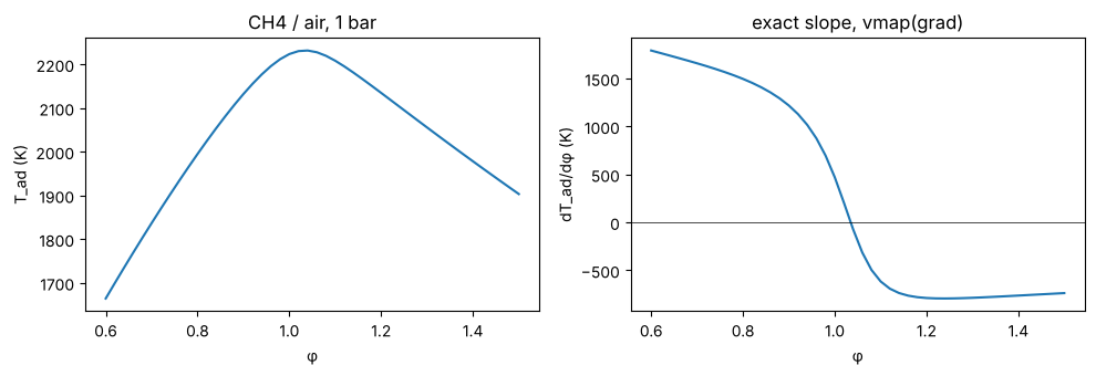
5. Adiabatic flame temperature of methane in air from gaspype’s species data, and its exact slope with respect to the equivalence ratio.

6. A reformer and water-gas-shift train, optimised by gradient.

Gaspype is optional: pip install gaspype or pip install "difflow[gaspype]".

import jax
jax.config.update("jax_enable_x64", True)
import jax.numpy as jnp
import numpy as np
import matplotlib.pyplot as plt
import gaspype as gp

from difflow import GibbsReactor, GibbsReactorParams, make_stream
from difflow.gaspype_import import GaspypeThermo, list_available_species

print("gaspype", gp.__version__, "-", len(list_available_species()), "gas-phase species")

gaspype 1.1.6 - 1057 gas-phase species

1. Gaspype on its own

A fluid_system fixes the species. A fluid is a composition over them, and gp.equilibrium returns the equilibrium fluid. Arrays of temperature broadcast, so one call solves a whole sweep.

Here 1 mol CH4 and 3 mol H2O (steam-to-carbon S/C = 3) are taken to equilibrium at 1 bar.

SMR = ["CH4", "H2O", "H2", "CO", "CO2"]
fs = gp.fluid_system(SMR)
feed = gp.fluid({"CH4": 1.0, "H2O": 3.0}, fs)

T_sweep = np.linspace(600.0, 1300.0, 71)
eq = gp.equilibrium(feed, T_sweep, 1e5)          # one vectorised call
x_gp = eq.array_fractions                        # (71, 5)

fig, ax = plt.subplots(figsize=(6, 3.5))
for i, s in enumerate(SMR):
    ax.plot(T_sweep - 273.15, x_gp[:, i], label=s)
ax.set(xlabel="T (°C)", ylabel="mole fraction", title="SMR equilibrium, S/C = 3, 1 bar (gaspype)")
ax.legend(); plt.tight_layout(); plt.show()

2. Gaspype’s JAX backend

With backend="jax", the arrays become jax.numpy arrays. An eager jax.grad differentiates through the unrolled Newton iterations, and it matches a finite difference. Under jax.jit the iteration is a lax.while_loop, and reverse mode through a while loop is not defined in JAX.

fs_jax = gp.fluid_system(SMR, backend="jax")

def x_h2_gaspype(T):
    eq = gp.equilibrium(gp.fluid({"CH4": 1.0, "H2O": 3.0}, fs_jax), T, 1e5)
    return eq.array_fractions[SMR.index("H2")]

h = 1e-2
print("eager grad      :", float(jax.grad(x_h2_gaspype)(1000.0)))
print("finite diff     :", float((x_h2_gaspype(1000.0 + h) - x_h2_gaspype(1000.0 - h)) / (2 * h)))
try:
    jax.jit(jax.grad(x_h2_gaspype))(1000.0)
except ValueError as e:
    print("jit(grad) fails :", str(e).splitlines()[0])

eager grad      : -1.8393047819920127e-05

finite diff     : -1.8407170332412903e-05
jit(grad) fails : Reverse-mode differentiation does not work for lax.while_loop or lax.fori_loop with dynamic start/stop values. Try using lax.scan, or using fori_loop with static start/stop.

So gaspype’s own solver is good for forward sweeps and quick eager gradients. It cannot sit inside a compiled, differentiated difflow model.

3. Gaspype data in difflow’s GibbsReactor

GaspypeThermo(species) exposes gaspype’s data the way GibbsReactor wants it: names, gibbs(T), enthalpy(T) and ELEMENTS. By default (method="nasa9") it evaluates the NASA-9 polynomials in jax.numpy, so H and G are smooth in T. method="table" instead uses gaspype’s public fluid_system, which interpolates linearly on a 1 K table. That table makes dG/dT piecewise constant.

Species names are gaspype’s, and they become the stream keys (F_CH4, …).

th = GaspypeThermo(SMR)
print(th.names, {e: v.tolist() for e, v in th.ELEMENTS.items()})

def reformer(T, P=1e5, S_C=3.0):
    inlet = make_stream({"CH4": 1.0, "H2O": S_C}, T=900.0, P=P)
    return GibbsReactor(GibbsReactorParams(thermo=th, T_out=T))(inlet)

out, info = reformer(1000.0)
print("converged:", bool(info["converged"]), " duty:", float(info["heat_duty"]) / 1e3, "kW per mol/s CH4")

('CH4', 'H2O', 'H2', 'CO', 'CO2') {'C': [1.0, 0.0, 0.0, 1.0, 1.0], 'H': [4.0, 2.0, 2.0, 0.0, 0.0], 'O': [0.0, 1.0, 0.0, 1.0, 2.0]}

converged: True  duty: 227.00842072761012 kW per mol/s CH4

The two solvers use the same species data. Gaspype’s 1 K table is exact at whole kelvins, which is where this sweep lands, so the equilibria agree to solver tolerance. Between whole kelvins, the table’s linear interpolation differs from the polynomials by about 0.1 J/mol.

def fractions(T):
    out, _ = reformer(T)
    n = jnp.array([out[f"F_{s}"] for s in SMR])
    return n / n.sum()

x_df = jax.jit(jax.vmap(fractions))(jnp.asarray(T_sweep))
print("max |x_difflow - x_gaspype| over the sweep:", float(jnp.max(jnp.abs(x_df - x_gp))))

max |x_difflow - x_gaspype| over the sweep: 9.492406860545088e-15

4. Compiled gradients

difflow gets dz/dθ from one Newton correction at the converged point, the implicit function theorem. It does not unroll the solve, so the derivative of the H2 fraction with respect to T, P and S/C can be compiled. It matches a central difference.

The check is at 1050 K, not 1000 K. Most species switch NASA-9 polynomials at 1000 K, and the two fits do not quite meet there: G steps by about 0.01-0.02 J/mol. A ±0.01 K difference that straddles the join measures that step, not the slope.

def x_h2(T, P, S_C):
    out, _ = reformer(T, P, S_C)
    n = sum(out[f"F_{s}"] for s in SMR)
    return out["F_H2"] / n

T0 = 1050.0
g = jax.jit(jax.grad(x_h2, argnums=(0, 1, 2)))(T0, 1e5, 3.0)
fd = [(x_h2(T0 + 1e-2, 1e5, 3.0) - x_h2(T0 - 1e-2, 1e5, 3.0)) / 2e-2,
      (x_h2(T0, 1e5 + 10.0, 3.0) - x_h2(T0, 1e5 - 10.0, 3.0)) / 20.0,
      (x_h2(T0, 1e5, 3.0 + 1e-5) - x_h2(T0, 1e5, 3.0 - 1e-5)) / 2e-5]
for name, a, b in zip(["dx/dT (1/K)", "dx/dP (1/Pa)", "dx/d(S/C)"], g, fd):
    print(f"{name:13s} jit(grad) = {float(a): .6e}   central diff = {float(b): .6e}")

dx/dT (1/K)   jit(grad) = -8.687206e-05   central diff = -8.687206e-05
dx/dP (1/Pa)  jit(grad) = -2.626973e-08   central diff = -2.626973e-08
dx/d(S/C)     jit(grad) = -7.267835e-02   central diff = -7.267835e-02

5. Adiabatic flame temperature

Gaspype’s database supplies the radicals and minor species a flame needs. Here methane burns in air (O2 + 3.76 N2) at equivalence ratio φ. The reactor is adiabatic, so the outlet temperature is an unknown of the Newton solve. jax.vmap of jax.grad gives the exact slope dT_ad/dφ along the curve.

FLAME = ["CH4", "O2", "N2", "H2O", "CO2", "CO", "H2", "OH", "H", "O", "NO"]
th_flame = GaspypeThermo(FLAME)
burner = GibbsReactor(GibbsReactorParams(thermo=th_flame, mode="adiabatic"))

def T_ad(phi):
    o2 = 2.0 / phi
    out, info = burner(make_stream({"CH4": 1.0, "O2": o2, "N2": 3.76 * o2}, T=298.15, P=1e5))
    return info["T"]

phis = jnp.linspace(0.6, 1.5, 46)
T_curve = jax.jit(jax.vmap(T_ad))(phis)
dT_curve = jax.jit(jax.vmap(jax.grad(T_ad)))(phis)
i_max = int(jnp.argmax(T_curve))
print(f"peak T_ad = {float(T_curve[i_max]):.0f} K at phi = {float(phis[i_max]):.2f}")

fig, ax = plt.subplots(1, 2, figsize=(10, 3.5))
ax[0].plot(phis, T_curve); ax[0].set(xlabel="φ", ylabel="T_ad (K)", title="CH4 / air, 1 bar")
ax[1].plot(phis, dT_curve); ax[1].axhline(0, color="k", lw=0.5)
ax[1].set(xlabel="φ", ylabel="dT_ad/dφ (K)", title="exact slope, vmap(grad)")
plt.tight_layout(); plt.show()

peak T_ad = 2232 K at phi = 1.04

6. Reformer + shift, optimised by gradient

A two-reactor train: an isothermal reformer at T_ref, then a water-gas-shift reactor at 600 K that is limited to the shift reaction (reactions=[{"CO": -1, "H2O": -1, "CO2": 1, "H2": 1}]). Methane that slips past the reformer does not react in the shift.

The objective is a toy margin per mol/s of methane: H2 product, minus the reformer heat duty and the steam raised, both priced in H2-equivalents. The design variables are T_ref and S/C. The gradient comes from jax.value_and_grad through both equilibrium solves, and a few Adam steps are enough.

shift = GibbsReactor(GibbsReactorParams(thermo=th, T_out=600.0,
                                        reactions=[{"CO": -1, "H2O": -1, "CO2": 1, "H2": 1}]))
C_HEAT = 1.0 / 286e3      # mol H2 per J of reformer duty (H2 HHV)
C_STEAM = 0.15            # mol H2 per mol steam raised

def margin(x):
    T_ref, S_C = x
    out1, info1 = GibbsReactor(GibbsReactorParams(thermo=th, T_out=T_ref))(
        make_stream({"CH4": 1.0, "H2O": S_C}, T=800.0, P=1e5))
    out2, _ = shift(out1)
    return out2["F_H2"] - C_HEAT * info1["heat_duty"] - C_STEAM * S_C

vg = jax.jit(jax.value_and_grad(margin))
x = jnp.array([950.0, 2.0])
scale = jnp.array([50.0, 0.5])          # step sizes in each variable's own units
m, v = jnp.zeros(2), jnp.zeros(2)
hist = []
for k in range(1, 151):                 # Adam on the scaled variables (ascent)
    f, g = vg(x)
    g = g * scale
    m = 0.9 * m + 0.1 * g; v = 0.999 * v + 0.001 * g**2
    step = (m / (1 - 0.9**k)) / (jnp.sqrt(v / (1 - 0.999**k)) + 1e-12)
    x = x + 0.05 * scale * step
    hist.append(float(f))
f, g = vg(x)
print(f"T_ref = {float(x[0]):.1f} K, S/C = {float(x[1]):.3f}, margin = {float(f):.4f} mol H2 per mol CH4")
print("gradient at the end:", np.asarray(g))

fig, ax = plt.subplots(figsize=(5, 3))
ax.plot(hist); ax.set(xlabel="iteration", ylabel="margin (mol H2 eq / mol CH4)"); plt.tight_layout(); plt.show()

T_ref = 1024.7 K, S/C = 2.619, margin = 2.5414 mol H2 per mol CH4
gradient at the end: [ 7.03142636e-09 -1.32525848e-04]

Summary

• Gaspype can be used with difflow. difflow.gaspype_import.GaspypeThermo adapts its gas-phase species database to GibbsReactor in a few lines. The equilibria match gaspype’s own solver, and the gradients compile.

• Gaspype’s own JAX solver is fine for forward sweeps and eager jax.grad. It cannot be differentiated under jax.jit, because of its while_loop. Use the adapter wherever difflow needs a gradient.

• What the adapter does not cover. It is ideal gas only. Gaspype has no liquids in a fluid, no VLE and no critical properties. It does have condensed species for activity calculations, but the adapter does not use them. The default "nasa9" path reads gaspype’s private database reader, so a future gaspype release could move it. method="table" uses only the public API, but its T derivatives are piecewise constant.