Lecture 18: Context engineering, tools, search and retrieval#
At a glance
Session Lecture 18, Week 9
Arc LLM and agentic engineering
Slides Deck for this session
Practice Practice module for this session
Demo
l18-context-engineering.ipynb, five retrievers over the L1 to L17 notes measured on 28 labelled questions; the deck’s capstone answers questions about the notes in your browserTools SQLite FTS5, sentence-transformers, FAISS, PyLate; in the browser, MiniSearch, transformers.js and WebLLM
Assignment None released with this session
Why this matters#
In November 2022 a man named Jake Moffatt asked the chatbot on Air Canada’s website about bereavement fares after his grandmother died. The chatbot told him he could buy a full-price ticket now and apply for the reduced fare afterwards. The airline’s own “Bereavement travel” page, which the chatbot’s answer linked to, said, in the tribunal’s summary, that the policy does not apply to requests for bereavement consideration after travel has been completed. He flew, applied, and was refused. In February 2024 the Civil Resolution Tribunal of British Columbia found the airline liable for negligent misrepresentation and awarded $650.88 (Moffatt v. Air Canada, 2024 BCCRT 149). Air Canada had argued that the chatbot was responsible for its own statements, which the tribunal called “a remarkable submission.” It also found that there was “no reason why Mr. Moffatt should know that one section of Air Canada’s webpage is accurate, and another is not.”
The decision does not say how the chatbot was built, and these notes do not guess. The useful fact for an engineer is narrower: the authoritative passage existed, on the same website, and the answer was not built from it. An LLM answers from whatever text is in its context window when it generates, plus what it absorbed in training. If the right passage is not in the window, the model does not know it is missing; it writes a fluent answer anyway, as L17 showed it must.
This session is about putting the right text in the window. That work now has a name, context engineering, and most of it is retrieval: fetching files and web pages with tools, searching a document store by keyword, searching it by meaning, sorting the results, and deciding when nothing found is good enough to use. Everything is measured on one corpus every student has read part of: the course’s own notes for L1 to L17. The session ends with that corpus answering questions about itself, in the deck, in your browser.
Learning objectives#
By the end of this session you should be able to:
Explain context engineering: an LLM answers from what is in its context window, so deciding what goes there, and how it gets there, determines the answer.
Give a model a tool, explain the tool-call exchange, and recognize when fetching context on demand (reading files, searching the web) is the right design, and the prompt-injection risk it brings.
Build keyword search (an inverted index with BM25) and semantic search (embeddings), combine them, and rerank the result with a cross-encoder; explain where late interaction (ColBERT) sits between them.
Choose chunk size, embedding model and index from measured trade-offs in hit rate, memory and search time, and say what changes when the index moves to a server.
Assemble a grounded prompt with citations within a token budget, and measure retrieval with hit@k and MRR on a gold set of queries.
Trace each stage of a retrieval pipeline running in the browser: what runs at build time, what runs on the page, and what each costs.
The context window decides the answer#
A model’s context window holds everything it reads before it writes: the system instructions, the conversation so far, any documents or tool results placed there, and the question. L17 treated it as a budget in tokens, money and latency. Here it is also the only channel through which your documents reach the model at the moment it answers.
Definition: context engineering
Context engineering is choosing what goes into a model’s context window, and building the machinery that gets it there, so that the right information is present when the model answers.
Anthropic’s engineering team puts it as “the set of strategies for curating and maintaining the optimal set of tokens (information) during LLM inference, including all the other information that may land there outside of the prompts” (Anthropic, 2025). Prompting, from L17, is the part you write by hand. Context engineering is the rest: the passages, the tool results, the history, and the decisions about what to leave out.
There are two ways to get text into the window. The model can fetch it on demand, calling tools that read a file or search the web while it works. Or your code can retrieve it in advance, searching an index of documents for passages related to the question and placing them in the prompt, which is called retrieval-augmented generation (RAG; Lewis et al., 2020). Most of this session is the second, because it is where the engineering decisions are, but the first is often the simpler design, and it comes first.
More context is not automatically better. Liu et al. (2024) placed the one relevant document at different positions among twenty and found a “U-shaped performance curve”: models used information at the start and end of a long context better than information in the middle. For one model, accuracy with the answer in the middle fell below its accuracy with no documents at all, 56.1%. Filling the window with everything that might matter is a way of hiding the part that does.
Fetching context with tools#
A tool is a function your code exposes to the model, described by a name, a sentence of
description and a JSON Schema for its arguments. The exchange is short. You send the tool
definitions with the request. If the model decides it needs the tool, it stops and returns a
request instead of an answer: the tool’s name and arguments, in Anthropic’s API a tool_use
block. Your code runs the function and sends the output back as a tool_result, and the model
continues, now with that output in its context
(tool-use documentation).
The model never runs anything itself. It writes a request; your code decides whether to honour it.
tools = [{
    "name": "read_file",
    "description": "Return the text of a file in the course repository.",
    "input_schema": {"type": "object",
                     "properties": {"path": {"type": "string"}},
                     "required": ["path"]},
}]
# The model replies with a tool_use block {"name": "read_file", "input": {"path": "..."}};
# your code reads the file and returns its text as a tool_result in the next message.
Reading files and searching the web#
The tools that fetch context are the familiar ones: list files, search them for a pattern, read one. Coding agents work this way. Given a repository, they grep for a function name, read the files that mention it, and follow references, instead of searching a precomputed index. A developer on Claude Code wrote that it “doesn’t use RAG currently. In our testing we found that agentic search out-performed RAG for the kinds of things people use Code for” (Hacker News comment, 2025). That is an informal statement by one team about code, not a benchmark, and it makes sense for code in particular: identifiers are exact, the files change constantly so an index goes stale, and grep is precise.
Web search and fetch tools bring in information that is newer than the model’s training data and that no local index holds. The provider runs the search and returns result snippets, or your code fetches a page and returns its text.
Model Context Protocol#
Every application used to wire up its own tools. The Model Context Protocol (MCP), introduced by Anthropic in November 2024 and now an open specification (modelcontextprotocol.io, current version 2026-07-28), standardizes the connection: a server exposes tools (functions the model can call), resources (data the application can read into the context) and prompts (templates), over JSON-RPC, and any client that speaks the protocol can use them. A file-system server, a database server or a search server written once works with every MCP client.
Text that gives orders#
Fetched text is untrusted input that the model reads as language. A web page, a PDF or a retrieved document can contain instructions aimed at the model (“ignore the previous instructions and…”). Greshake et al. (2023) demonstrated this indirect prompt injection against deployed LLM applications: the attacker never talks to the model; they plant text where the application will retrieve it. Nothing in the model reliably separates the instructions you wrote from instructions that arrived in a tool result. The defences are in the system around it: tools that cannot do damage (read-only by default), a person approving anything that writes or spends, and treating every fetched string as data.
What a practitioner should take from this
Fetch on demand when the source is precise and changing (a repository, a live system, the web) and the question tells you where to look. Retrieve from an index when the corpus is large, stable, and searched by meaning.
Every tool result enters the context window and costs tokens. Return what is needed, not whole files.
Assume every fetched document may contain instructions. Decide in code what a tool may do.
Keyword search over a document store#
Keyword search finds the passages that contain the words of the question, and ranks them by how strongly; it matches words, not meaning. It runs on an inverted index: a table from each word to the list of passages that contain it, with counts. A query looks up its words and scores only the passages they point to, which is why keyword search over millions of documents takes milliseconds. It is the index at the back of a textbook, built by a program.
BM25, written out#
The standard scoring function is BM25, from the probabilistic relevance framework of Robertson and colleagues (Robertson and Zaragoza, 2009, an author’s copy). A passage’s score is a sum over the query’s words:
Three ideas are packed into it. Inverse document frequency \(\text{idf}(t)\) makes rare words count more: “SiNDAE” appears in one passage of the notes and identifies it; “model” appears in most and identifies nothing. Term frequency \(f(t, d)\) counts the word in the passage, but the fraction saturates: the tenth “pump” adds far less than the first, and \(k_1\) sets how fast. Length normalization divides by the passage length relative to the average, so a long chapter is not rewarded just for containing more words; \(b\) sets how much. Robertson and Zaragoza report \(1.2 < k_1 < 2\) and \(0.5 < b < 0.8\) as reasonable in many settings; SQLite’s FTS5 fixes \(k_1 = 1.2\) and \(b = 0.75\) (FTS5 documentation).
The figure above splits each passage’s score into one bar segment per query word. With the query “pump suction pressure”, the long troubleshooting chapter says “pump” twelve times and still ranks second, because saturation and length normalization stop repetition from paying. Set \(b\) to 0 and it moves up; set \(k_1\) near 0 and only presence counts.
In a database#
You rarely write BM25 yourself. SQLite, which every Python install already has, builds an inverted index in a virtual table and ranks with BM25. This is the L3 database doing a new job:
db.execute("CREATE VIRTUAL TABLE notes USING fts5(body, tokenize='porter unicode61')")
db.executemany("INSERT INTO notes(rowid, body) VALUES (?, ?)", enumerate(texts))
db.execute("SELECT rowid FROM notes WHERE notes MATCH ? ORDER BY bm25(notes) LIMIT 5",
           ('"zero_grad"',))
bm25() returns smaller numbers for better matches, so an ascending sort puts the best first.
Postgres has the same machinery (tsvector, ts_rank), and Elasticsearch and OpenSearch are
built on it.
What keyword search finds and misses#
On the course notes, split into 516 section chunks, BM25 was scored against 28 questions written for this session, each labelled by hand with the sections that answer it. Two numbers summarize a retriever over the 24 answerable questions: hit@5, the fraction of questions with a relevant section among the top five, and MRR@10, the mean of one over the rank of the first relevant section, which rewards putting it first. My hand-written BM25 and SQLite’s FTS5 gave identical results: hit@5 of 0.83 and MRR@10 of 0.72.
The breakdown by kind of question explains the number. On the eight identifier questions, which name a function, a
library or a metric (zero_grad, GroupKFold, MAPIE, SiNDAE), BM25 found the answer every time:
rare tokens have a high idf. On the twelve paraphrase questions, which describe an idea in
words the notes do not use, it found only two thirds. “Adding up money in the database gave
answers that were off by a fraction of a cent” shares almost no words with the L3 section titled
“numeric versus double precision”; BM25 ranked that section fourteenth, behind sections that
happened to say “database” and “answers.” Keyword search matches vocabulary, and people asking
questions use their own.
Semantic search#
Semantic search matches meaning instead of words, using the sentence embeddings of L17. Each passage is embedded once, when the index is built; a question is embedded the same way when it is asked; and the passages whose vectors have the highest cosine similarity to the question’s are returned. The model that does this is a bi-encoder: it encodes the question and the passage separately, which is what lets the passage vectors be computed ahead of time.
Definition: bi-encoder
A bi-encoder embeds a query and a passage independently into vectors and scores the pair by their similarity, so every passage can be embedded once, in advance, and searched by vector comparison.
Chunking#
Before anything is embedded the documents are cut into chunks, the units that get retrieved. The course notes are cut at their H2 and H3 headings, one idea per section, and a section longer than 350 words is split again at paragraph boundaries with its heading repeated at the top. The repeated heading is there for the embedding model. The model used here, all-MiniLM-L6-v2, reads at most 256 word pieces and silently truncates the rest, so it sees roughly the first 200 words of a chunk. Putting “Evaluating on time / Why a shuffled split leaks” first means the part it reads says what the chunk is about. The tuning section below measures the alternatives.
Exact search is fast at this size#
The 516 chunks embed to 516 vectors of 384 numbers, 0.79 MB as 32-bit floats, in about 15 to 30 seconds on a laptop CPU. A question is one more embedding and one matrix product, about 1.5 ms. With fewer than a few hundred thousand chunks there is no reason to use anything cleverer than exact search, and every reason not to: an approximate index can only lose results.
The map above projects the 516 vectors to two dimensions, which keeps only about 11% of their variance, so treat it as a shadow. Sections of the same lecture mostly cluster, the database lectures in one region, the machine-learning lectures in another. The lines from a question run to its five nearest sections measured in all 384 dimensions, which is why some look long.
What embeddings find and miss#
Embedding search scored hit@5 of 0.88 and MRR@10 of 0.72. It found the money question’s answer at
rank 2, where BM25 had it at 14, and raised the paraphrase hit rate from 0.67 to 0.83. It lost
something too: one identifier question, and “why does the chatbot confidently invent a part number
that does not exist,” which BM25 answered at rank 1 because “part number” is in the L17 section and
which the embedding ranked fourteenth. L17’s warnings apply: an embedding does not know that
zero_grad and zero_grad() are the same token sequence, does not see units, and does not handle
negation.
Hybrid search#
The two retrievers fail on different questions, so combine them. Their scores live on unrelated scales (a BM25 score of 12 and a cosine of 0.5 cannot be added), so the standard combination uses ranks only. Reciprocal rank fusion gives each passage \(1/(60 + r)\) for its rank \(r\) in each list and sums (Cormack, Clarke and Buettcher, 2009, an author’s copy, where \(k = 60\) “was fixed during a pilot investigation”). A passage near the top of either list scores well; a passage near the top of both scores best.
Hybrid search scored hit@5 of 0.92 and MRR@10 of 0.77, better than either retriever alone, and recovered every identifier question while keeping the paraphrase gains. It also shows why the top-ranked passage deserves suspicion. For “why can’t I shuffle sensor readings before splitting them into training and test sets,” fusion ranked first the L12 section on why a transformer ignores the order of shuffled tokens, and put the correct L8 section on leakage second. Both retrievers liked the L12 passage for the word “shuffle.” A model that leans on passage [1] answers the wrong question.
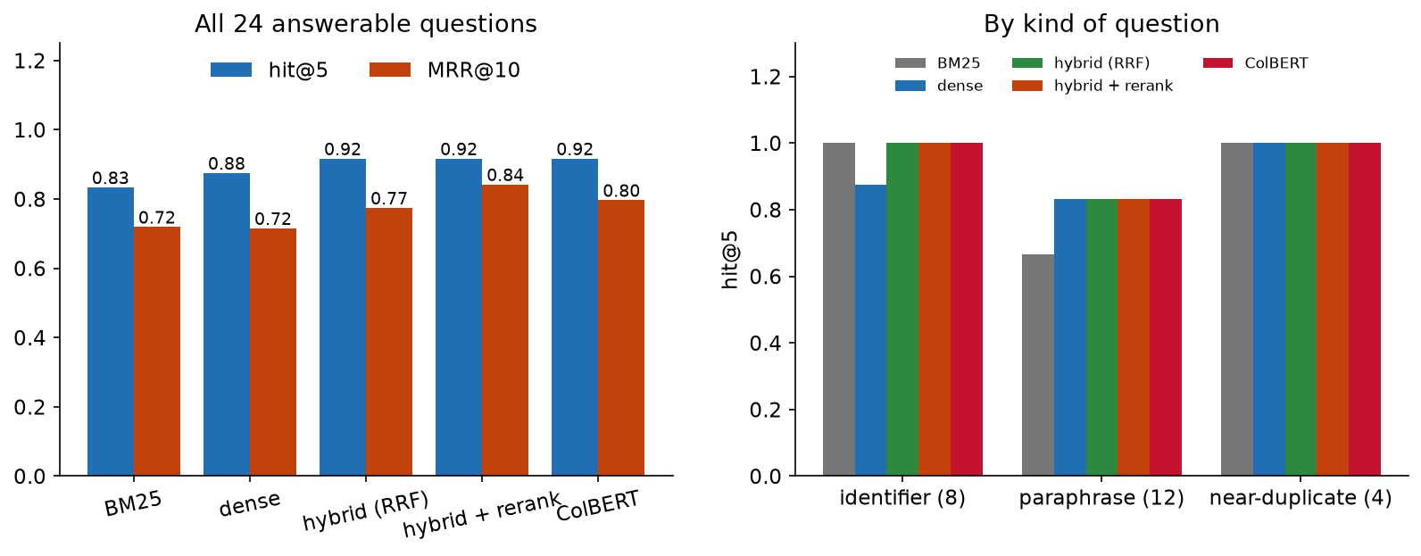
Fig. 138 Five retrievers over the 516 sections of the L1 to L17 notes, scored on the 24 answerable gold
questions. With 24 questions one question moves hit@5 by 0.04. Generated by
figures/make_figures.py; the notebook prints the same numbers.#
Re-ranking and late interaction#
A bi-encoder compresses a whole passage into one vector before it has seen the question, so it cannot attend to the particular words the question cares about. A cross-encoder reads the question and the passage together, as one input, and outputs a relevance score for the pair. It is more accurate and cannot be precomputed: every new question needs a fresh pass over every passage you want to score. Reimers and Gurevych (2019) put the difference in numbers for a related task, finding the most similar pair among 10,000 sentences: about 65 hours with a cross-encoder, about 5 seconds with a bi-encoder.
Definition: cross-encoder
A cross-encoder reads a query and a passage together as one input and outputs a relevance score for the pair; it is more accurate than comparing separate embeddings, but must run once per pair at query time.
So the two are used in sequence: the cheap retrievers produce 20 to 50 candidates, and a cross-encoder re-ranks them (Nogueira and Cho, 2019, who reported a 27% relative improvement in MRR@10 on MS MARCO by reranking with BERT). Here ms-marco-MiniLM-L-6-v2 reranked the hybrid top 20. Hit@5 stayed at 0.92, since reranking cannot recover a passage that was not in the 20, and MRR@10 rose from 0.77 to 0.84: the right section moved up, usually to first. The shuffled split question’s L8 section went from rank 2 to rank 1.
Two costs come with it. Time: scoring 20 pairs took 1 to 2 seconds per question on a laptop CPU, a thousand times the cost of the search itself. And reranking can hurt: the money question’s section, ranked first by fusion, dropped to eighth. This reranker was trained on short web search queries, and long technical paraphrases are not what it learned.
Late interaction: ColBERT#
There is a design between the two. ColBERT (Khattab and Zaharia, 2020) keeps one vector for every token of a passage instead of one per passage, computed in advance like a bi-encoder. At query time each token of the question finds its most similar token in the passage, and the passage’s score is the sum of those maxima, an operation called MaxSim. The interaction between question and passage happens late, after both are encoded, which keeps the passage side precomputable while letting individual words match.
Definition: late interaction
Late interaction encodes the query and the passage separately into one vector per token, then scores the pair by matching each query token to its most similar passage token (MaxSim) and summing.
In the figure, each row is a token of “what happens if you forget zero_grad in a PyTorch training loop”, each column a token of the L11 section, and the dot marks each row’s best match: “forget” finds “forgot” at 0.89. The rows of [MASK] are query augmentation: ColBERT pads every query to 32 tokens and lets those padding vectors match too, and they contribute 11.6 of this passage’s score of 29.8.
The original paper reports reranking two orders of magnitude faster than BERT, 61 ms against 10,700 ms per query. On the course notes, answerai-colbert-small-v1 (run with PyLate) scored hit@5 of 0.92 and MRR@10 of 0.80, between hybrid search and reranking, at 12 ms per question with brute-force scoring. The cost is storage. One vector per token meant 96,905 vectors of 96 numbers, 37 MB, against 0.79 MB for one vector per chunk: 47 times more. ColBERTv2 compresses those vectors and reports a 6 to 10 times smaller footprint. Across many datasets, the BEIR benchmark found that “re-ranking and late-interaction-based models on average achieve the best zero-shot performances”, and that BM25 “is a robust baseline” that dense models “often underperform” (Thakur et al., 2021).
Tuning and scaling#
Every retrieval system makes the same handful of choices. None has a best value; each has a measurement.
Chunk size and overlap#
Small chunks retrieve precisely and lose context; large chunks keep context, dilute the topic, and overrun the embedding model’s input limit. Overlap, repeating the last part of one chunk at the start of the next, keeps an idea that spans a boundary from being cut in half, at the cost of more chunks. Libraries ship defaults, and their units differ: LangChain’s text splitter defaults to 4,000 characters with 200 of overlap, LlamaIndex’s sentence splitter to 1,024 tokens with 200 (LangChain source, LlamaIndex source). Neither source gives a reason for its numbers.
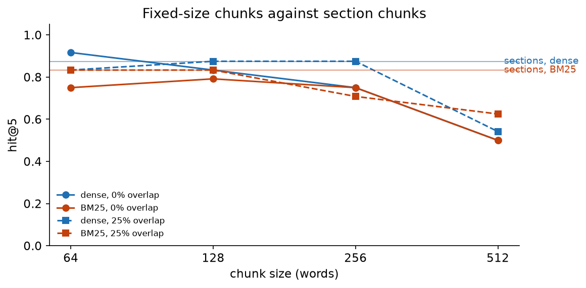
Fig. 139 Fixed-size word windows over the same notes, ignoring section boundaries, against section chunks.
A window counts as relevant if most of its words came from a relevant section. Generated by
figures/make_figures.py.#
The sweep cut the same notes into fixed windows of 64 to 512 words, with and without 25% overlap. At 512 words both retrievers fell to between 0.50 and 0.62: past the embedding model’s input limit, and too diluted for BM25. Between 64 and 256 words the results moved between 0.71 and 0.92 with no consistent winner and no consistent effect of overlap, which on 24 questions is within the noise of one or two questions. Section chunks matched the best of them (0.88 dense, 0.83 BM25) with a third as many chunks as 64-word windows, and each one is a complete, readable section that can be cited. Cut at the document’s own structure first; cap the size below the embedding model’s limit; then measure on your questions rather than adopting a default.
Choosing the embedding model#
The MTEB leaderboard (Muennighoff et al., 2023) ranks embedding models across many tasks and is the place to start a shortlist. The decision is made on your own gold set, weighing dimension (storage and speed), maximum input length (chunk size), domain, license, and whether the model runs locally or behind an API, which sends every document and question to the provider. Some models are trained so a vector can be truncated to fewer dimensions with little loss (Matryoshka representations; Kusupati et al., 2022), for example nomic-embed-text-v1.5. Switching models means re-embedding the whole corpus, and a query embedded with a different model from the index silently ruins retrieval, so the model name and version belong in the index’s metadata.
Memory and search time#
Memory is arithmetic: number of vectors × dimensions × bytes per number. One million 768-dimension vectors take 3.07 GB as 32-bit floats, 0.77 GB as 8-bit integers, and 96 MB as one bit per dimension. Quantizing costs some accuracy; a Hugging Face study measured int8 embeddings keeping about 97% of retrieval performance and binary about 92.5%, rising to about 96% when the top results are rescored with the full vectors (Shakir, Aarsen and Lee, 2024).
Search time is the other axis. Exact search compares the question with every vector, so its cost
grows with the corpus: on 100,000 vectors of 384 dimensions, about 13 to 16 ms per question on a
laptop CPU. Approximate nearest neighbor search gives up a little recall for a lot of speed.
The common index is HNSW (Malkov and Yashunin, 2020), a
layered graph in which a search walks from neighbor to neighbor toward the query; its search
breadth efSearch trades speed for recall.
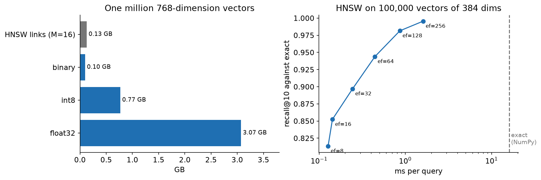
Fig. 140 Left: storage for one million vectors. Right: HNSW from FAISS on 100,000 synthetic vectors with
structure (384 dimensions generated from a 32-dimensional latent space), recall measured against
exact search, single-threaded. Generated by figures/make_figures.py.#
With FAISS (Douze et al., 2024), an HNSW index on those 100,000
vectors took under a minute to build. At efSearch 64 it answered in 0.44 ms with recall@10 of
0.944 against exact search, about 36 times faster; at 256, 1.6 ms and 0.996. The graph adds about
128 bytes per vector at the usual setting of 16 links per node, which for binary vectors is more
than the vectors themselves. Approximate search is the right tool past a few hundred thousand
chunks or under a tight latency budget, and the trade is always measured against exact search on
the same questions.
When the index moves to a server#
Until then, an index can live in the process: a NumPy array, FAISS, sqlite-vec, LanceDB or Chroma. When many users, a large corpus or continuous updates make that impractical, it moves to a server, and the choices fall into three groups.
Kind |
Examples |
What you get |
Watch for |
|---|---|---|---|
A database you already run |
Postgres with pgvector |
SQL, joins, transactions, roles and backups next to the vectors |
approximate indexes filter after the scan, so a restrictive filter returns too few rows |
A search engine |
OpenSearch, Elasticsearch |
BM25 and vector search in one engine, hybrid queries, document-level security |
operational weight; Elasticsearch’s license and feature tiers |
A vector database |
Qdrant, Weaviate, Milvus; Pinecone as a managed service |
filtering during graph search, quantization, scale-out |
another system to secure and operate |
The engineering changes on a server are mostly not about vectors. Authentication: API keys or database roles, TLS on every connection, and keys kept out of the code as in L1 and L2. Qdrant’s documentation is blunt that “self-hosted open source deployments are not secure by default” and that “connections are unencrypted by default” (Qdrant security). Permissions per document: a shared index with no filter lets anyone who can ask a question retrieve any document, so each chunk carries access metadata and every query filters on the user’s rights. Postgres can enforce this with row-level security, but pgvector’s own documentation warns that “with approximate indexes, filtering is applied after the index is scanned”, so a user allowed to see a tenth of the corpus gets about four results from a search for forty; partitioning by tenant avoids it. Updates and deletes: a revised standard must replace the old chunks, not sit beside them. And re-embedding: changing the model means rebuilding the whole index.
Assembling and measuring the context#
The last step puts the passages in the prompt. The capstone’s prompt, which the notebook also builds, has four parts: an instruction to answer only from the passages and cite them, the question, the top five passages numbered and labelled with their lecture and section, and the question again at the end, where a small model attends to it best. Each passage is cut to its first 120 to 220 words. Five passages and the instruction come to about 1,000 to 1,600 tokens, well inside the window and short enough that nothing important sits deep in the middle.
When to say “not in the notes”#
Four of the 28 gold questions are not answered anywhere in the notes: LoRA fine-tuning, the Kalman filter, Kubernetes and PagedAttention. Retrieval still returns five passages for each, because a search always returns its top five. Told to reply “Not in the notes” when the passages do not answer, a one-billion-parameter model in the capstone instead produced a confident definition of LoRA from passages about something else. Abstention has to be decided in code, from the retrieval scores, before the model is asked.
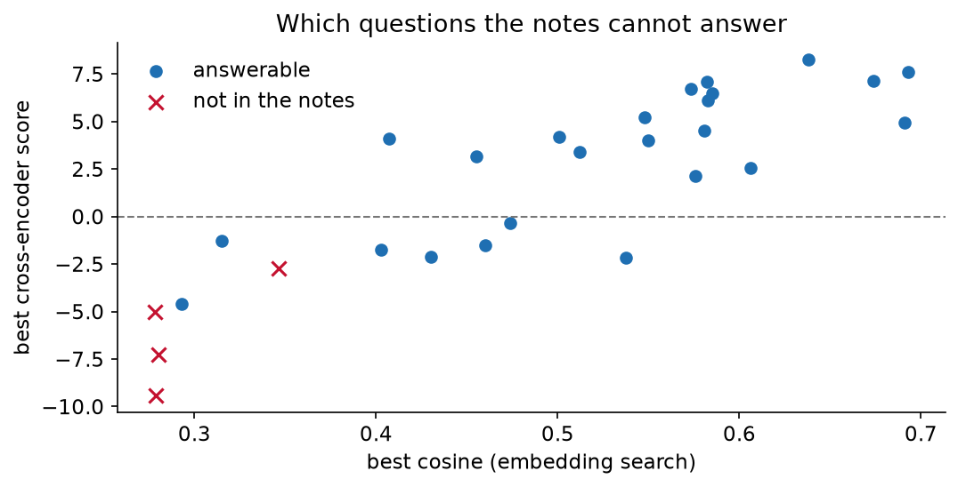
Fig. 141 The best cosine and best cross-encoder score for each gold question. The answerable and
unanswerable questions overlap. Generated by figures/make_figures.py.#
The scores overlap. The obvious rule, abstain when the cross-encoder’s score is below zero, would have refused seven answerable paraphrase questions. On this corpus, abstaining when the best cosine is below 0.285 or the best cross-encoder score is below −6 caught three of the four unanswerable questions and refused none of the answerable ones, and the Kalman filter question, at a cosine of 0.35, slipped through. The margins are a few hundredths. A threshold is a property of a corpus and two models, so it is calibrated on a gold set and recalibrated when any of them changes.
Building the gold set#
A gold set is a list of questions, each labelled with the passages that answer it, written by someone who knows the documents. Retrieval is measured on it before anyone reads a generated answer, because a correct answer built on a wrong passage is luck, and a wrong answer built on the right passage is a generation problem, not a retrieval one. The 28 questions here were written to cover each retriever’s strengths (identifiers, paraphrases, near-duplicate sections) and to include questions the notes cannot answer. With 24 answerable questions, one question moves hit@5 by 0.04; the differences in this session between hybrid search, reranking and ColBERT are within that.
Capstone: chat with the course notes#
The deck for this session ends with every block above running in one browser tab, answering questions about the released course notes and slides with no server and no API key.
At build time, in the course’s CI on every deploy: a script chunks the notes and slides of every released lecture, one chunk per section and one per slide, about 1,200 for L1 to L17, and embeds them with all-MiniLM-L6-v2 through transformers.js, the same library and settings the browser uses. The index, 1.9 MB with the vectors stored as 8-bit integers, is built from what the course has released and never committed, so an unreleased lecture can never be retrieved.
In the browser, for each question: BM25 over the chunks with MiniSearch (about 5 ms); the question embedded by transformers.js (about 25 ms); exact cosine against every chunk (about 3 ms); reciprocal rank fusion; an optional cross-encoder rerank of the top 12 (about 3 s); the gate; the prompt, shown verbatim; and generation by WebLLM, which runs a quantized model on the laptop’s GPU through WebGPU. Every stage is drawn as a block and timed.
The model is the slow, expensive and unreliable part. Qwen2.5 1.5B needs about 1.6 GB of GPU memory; its first download took about 13 minutes on the development network and later loads come from the browser cache in about 5 seconds; an answer takes about 25 seconds. On the shuffled-split question it gave a correct two-sentence answer in the passage’s own terms. Llama 3.2 1B, half the size, at first produced nothing but citation markers, then one correct answer and one that inverted the passage. One run each is an anecdote, and the chat is there to show the pipeline: read the passages and the prompt before trusting the answer.
Two details of the design limit who can use it. WebGPU is available only on secure (HTTPS) pages and in recent browsers (MDN); without it, the chat stops after assembling the prompt and shows the passages and links. And unlike the other interactive figures in these notes, which never touch the network, the chat downloads its libraries and model weights the first time they are needed, deliberately and only on request.
Limitations and trade-offs#
Retrieval sets a ceiling. The best retrievers here found a relevant section in the top five for 22 of 24 questions, and each missed a different pair. One question, “how can I tell whether the error bars my model reports can be trusted”, defeated all of them: its answer is in the L14 and L15 sections on calibration, which never use the words “error bars” or “trusted”, and no retriever placed them in the top five. A generator cannot cite a passage it was never given.
The top passage can be the wrong one. Keyword overlap put the L12 section on shuffled tokens above the L8 section on shuffled splits. Rerankers help and can also hurt, as the money question showed.
Small models read unreliably. A model that runs in a browser tab summarizes and quotes; it does not reason well, and it will answer when it should not. The gate and the visible prompt exist because of that.
Thresholds and gold sets are small and specific. The abstention thresholds have margins of a few hundredths, and 24 questions cannot separate methods that differ by one question.
Indexes go stale. A retrieved passage is only as current as the last rebuild. Fetching on demand avoids this and pays for it in latency and tokens.
Retrieved text is untrusted. Anything in the corpus or on the web can carry instructions.
Sometimes retrieval is the wrong tool. A small, stable corpus may fit in the context window: the L1 to L17 notes are about 107,000 words, roughly 140,000 tokens, which fits some long-context models, at the price of sending all of it with every question and the lost-in-the-middle effect. The choice between levers reduces to one table.
The problem |
The lever |
|---|---|
The model lacks knowledge that lives in your documents |
retrieval, or fetching with tools |
The documents are small and stable, and cost per question is acceptable |
the whole corpus in the context window |
The format or behavior is wrong, and the knowledge is fine |
a better prompt (L17), then fine-tuning |
The knowledge changes daily |
retrieval or tools, never fine-tuning |
In-class demo#
The notebook l18-context-engineering.ipynb builds the five
retrievers over the frozen L1 to L17 snapshot, BM25 by hand and in SQLite, embeddings, fusion, a
cross-encoder and ColBERT, and prints the ladder, the gate calibration, a chunk-size sweep, and
exact against approximate search on 100,000 vectors, ending with an assembled prompt. It runs on a
CPU in several minutes after downloading three small models. Then the capstone in the deck: ask it
about an earlier lecture, turn on reranking, and read the prompt it built.
Summary#
An LLM answers from its context window, so the quality of an answer is bounded by the passages put there. Context engineering is the work of choosing and fetching them: tools that read files and the web when the source is precise and changing, and retrieval from an index when the corpus is large and searched by meaning. On the course notes, keyword search found every question that named an identifier and two thirds of the paraphrases; embedding search found more paraphrases and lost some identifiers; fusing their rankings beat both; a cross-encoder put the right section first more often, at a thousand times the cost; and ColBERT matched them by storing a vector for every token. Chunk at the document’s structure, measure size and model choices on a gold set, use exact search until the corpus is large, and when the index moves to a server, treat authentication and per-document permissions as part of retrieval. Decide in code when the passages are too weak to answer from, because a small model will not. The capstone runs all of it in a browser tab, and its most useful output is the prompt.
Resources#
Moffatt v. Air Canada, 2024 BCCRT 149. The tribunal’s reasons, short and readable; the source for the opening case.
Anthropic, Effective context engineering for AI agents (2025). The term, and how agents manage what enters their context.
Lewis et al., Retrieval-Augmented Generation for Knowledge-Intensive NLP Tasks (NeurIPS 2020). The paper that named RAG.
Liu et al., Lost in the Middle (TACL 2024). Why more context is not automatically better.
Robertson and Zaragoza, The Probabilistic Relevance Framework: BM25 and Beyond (2009, author’s copy). BM25 from its authors, with what \(k_1\) and \(b\) mean.
SQLite FTS5. Full-text search in the database you already have.
Reimers and Gurevych, Sentence-BERT (EMNLP 2019). Bi-encoders against cross-encoders, with the cost numbers.
Nogueira and Cho, Passage Re-ranking with BERT (2019). The retrieve-then-rerank pattern.
Khattab and Zaharia, ColBERT (SIGIR 2020) and Santhanam et al., ColBERTv2 (NAACL 2022). Late interaction and its compression.
Thakur et al., BEIR (NeurIPS 2021). How retrievers transfer to new domains; why BM25 remains the baseline to beat.
Cormack, Clarke and Buettcher, Reciprocal Rank Fusion (SIGIR 2009, author’s copy). Two pages; the fusion rule used here.
Malkov and Yashunin, HNSW (TPAMI 2020) and The Faiss library. Approximate search and the library most others build on.
Hugging Face, Binary and Scalar Embedding Quantization (2024). Memory against accuracy, measured.
pgvector and Qdrant security. Vector search in Postgres, and what “not secure by default” means for a vector database.
Model Context Protocol specification. The standard interface for tools and resources.
Greshake et al., indirect prompt injection (2023). Attacks through retrieved content.
WebLLM and transformers.js. The two libraries that run the capstone in the browser.
Assignment#
No assignment is released with this session.
Practice module#
Practice module for this session, for participation credit.