Lecture 11: Tensors, autodiff, training loops, and GPUs#
At a glance
Session Lecture 11, Week 6
Arc Machine learning and deep learning
Slides Deck for this session
Practice Practice module for this session
Demo
l11-tensors-autograd.ipynb, a gradient by hand, a loop by hand, and three ways to break itStories
l11-four-models.ipynb, the four models that looked fine, rerun so you can dig into each
Why this matters#
For five weeks this course has been about the parts of a machine learning system that are not
the model. This session is where you finally write the model. Lecture 9 wrote
training as an optimization problem, minimizing a loss over the weights, and let scikit-learn’s
fit solve it out of sight. This session opens that solver. Automatic differentiation computes
the gradient, and the training loop is the optimizer written out by hand. It comes this late
because a training loop is about fifteen lines of code, and there are at least six ways to get it
silently wrong.
Here is one of them, measured on this session’s data. A small neural network is trained to
predict the compressive strength of concrete from its recipe. The code runs to completion, the
training loss falls steadily, and no exception is raised. The validation error comes out at
17.7 MPa. Predicting the average strength of the training set for every mix, which needs no
model at all, scores 17.9 on the same rows. The network has learned a constant. The cause is one
missing [:, None] on the target, and with it restored the same code scores 5.5 MPa.
PyTorch did print a warning about it, once per batch, and a notebook shows a repeated warning
only once, above a cell of output that looks like training.
Deep learning frameworks differ from the other tools in this course because they do not tell you
when a computation is wrong. A database rejects a malformed query, and a schema check fails
loudly. loss.backward() differentiates whatever graph you built, including one you built by
accident, and optimizer.step() applies the result. The framework does not check whether the
graph is the one you meant, so you have to understand what those calls do. So this
session starts from the mathematics of the gradient, looks at how the two major frameworks,
PyTorch and JAX, organize that mathematics
differently, and then works through five results that looked fine and were not: a gradient
check and four trained models.
The second argument is about expectations. A widespread assumption holds that a neural network is strictly more powerful than a gradient-boosted tree, and that engineers’ tabular datasets are simply too small to show it. On this session’s data, a fair comparison does not support that assumption. Getting to it requires the split discipline from Lecture 9.
Learning objectives#
By the end of this session you should be able to:
Explain what a backward pass computes by applying the chain rule to a small network, and why reverse mode suits a scalar loss better than finite differences.
Contrast how PyTorch (a recorded tape that accumulates into
.grad) and JAX (transformations of pure functions) compute the same gradient, and use that to explainzero_grad(),no_grad()and immutable arrays.Work with tensor shapes, broadcasting, dtypes and devices, and read a shape error.
Write a training loop in PyTorch and in JAX, and say what each of Adam’s hyperparameters does.
Diagnose a training failure that raises no error by comparing against an exact reference, the predict-the-mean baseline, or a grouped split.
Measure whether an accelerator helps before moving a model onto one.
Automatic differentiation#
Deep learning works because you can compute the gradient of a scalar loss with respect to millions of parameters, exactly, for roughly the cost of two forward passes. The technique is automatic differentiation, and it is neither symbolic algebra nor a numerical approximation. It is the chain rule, applied mechanically to the sequence of operations your code actually performed.
Definition: automatic differentiation
Automatic differentiation computes exact derivatives of a program by applying the chain rule to each elementary operation the program executes, and combining the local derivatives.
Take a network small enough to differentiate by hand: one hidden layer, a tanh activation, a
scalar output, and a squared-error loss on one example.
Here \(x\) is one input vector and \(y\) its measured target, the data. \(W\) and \(b\) are the hidden layer’s weight matrix and bias, \(v\) and \(c\) the output layer’s weight vector and bias, and these four are the parameters training adjusts. \(z\) and \(a\) are vectors with one entry per hidden unit, and \(\hat{y}\) is the scalar prediction. The chain rule gives every gradient in a few lines, and each step reuses the quantity computed by the step before it.
The graph, forward and backward#
The reuse is easiest to see as a graph. Each box below is an intermediate value, and each blue arrow is one operation from the forward pass. To run the backward pass, start from \(\partial L / \partial L = 1\) at the right, since the loss changes one-for-one with itself, and walk the red arrows to the left. Each red edge carries the local derivative of the forward step it reverses, such as \(\times\, v\) for \(\hat{y} = v \cdot a + c\). The gradient at a node is the gradient arriving from its right times the factor on the edge, which is the chain rule applied one step at a time. The quantity carried backwards, \(\partial L / \partial a\) at node \(a\), is called the adjoint of that node. Many texts write it \(\bar{a}\); these notes write the derivative out.
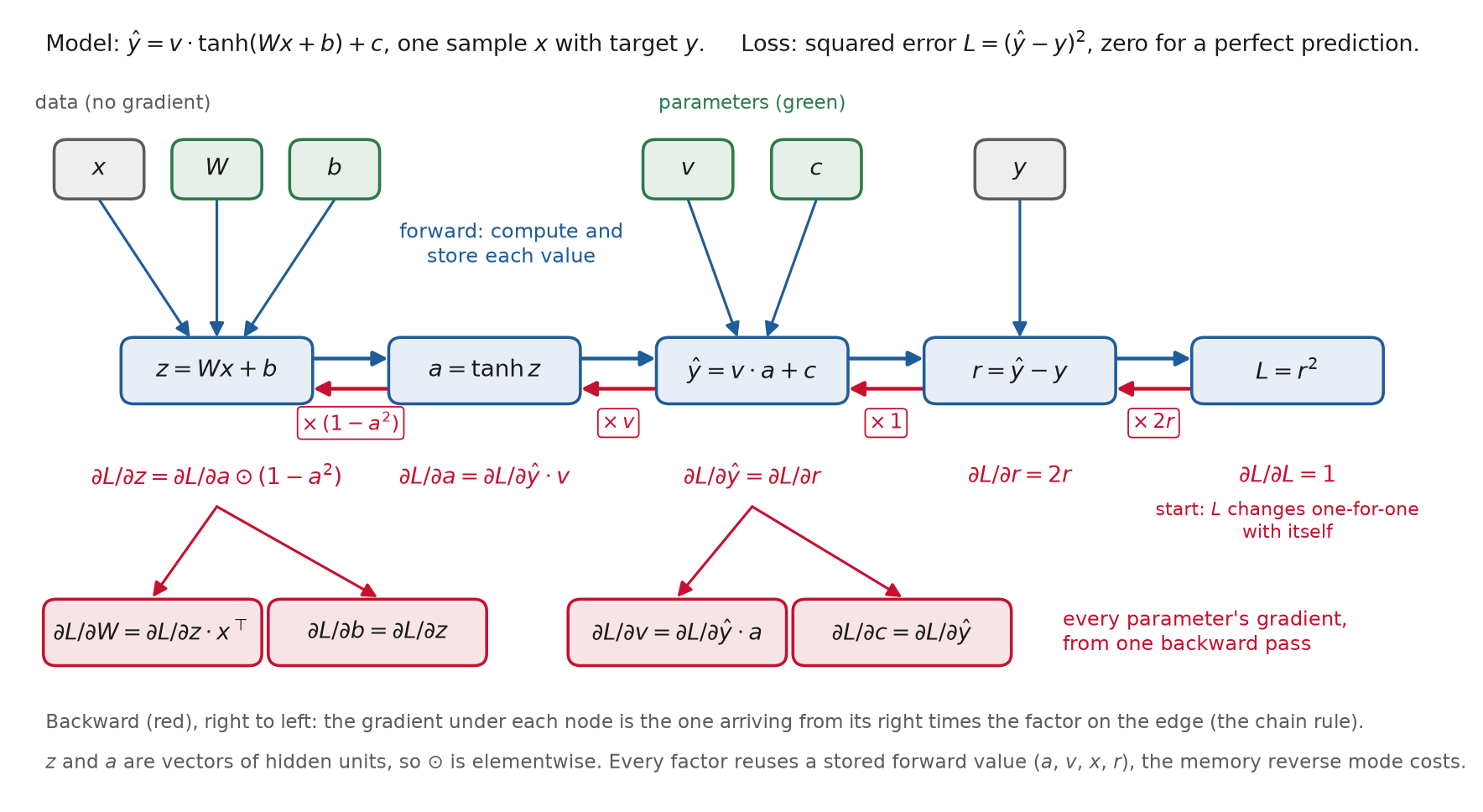
Fig. 65 The network above as a computation graph. The forward pass (blue) computes and stores each
intermediate. The backward pass (red) starts from \(\partial L / \partial L = 1\) and multiplies by
one local derivative per edge. The factor \(1 - a^2\) needs the stored \(a\), and
\(\partial L / \partial W\) needs the stored \(x\), which is why reverse mode costs memory. Drawn by figures/make_figures.py.#
Reverse-mode automatic differentiation is this computation, organized. Run the forward pass and keep each intermediate. Then walk the recorded operations backwards, multiplying by each local derivative. Because the loss is a scalar, one backward walk produces the derivative with respect to every parameter at once. Its cost is a small constant multiple of the forward pass, whether the model has nineteen parameters or nineteen million. In deep learning this is called backpropagation, a name that predates the general technique’s adoption in the field; the survey by Baydin and colleagues traces both histories.
Forward mode and reverse mode#
The chain rule can be accumulated in either direction, and the choice sets the cost. Forward mode pushes a derivative forward alongside the values, from one input direction at a time, so it costs one pass per input. Reverse mode pulls a derivative back from one output at a time, so it costs one pass per output. A training loss has millions of inputs (the parameters) and one output, so reverse mode wins by a factor of the parameter count. A simulator with three design variables and a thousand outputs is the opposite case, and forward mode is then the right tool.
Both frameworks expose both modes. In JAX they are jax.jvp (forward, a Jacobian-vector
product) and jax.vjp (reverse, a vector-Jacobian product), and jax.jacfwd and jax.jacrev
build full Jacobians from them. PyTorch has the same pair in torch.func.jvp and
torch.func.vjp, alongside the reverse-mode backward() most code uses. You will rarely call
these directly, but the distinction explains why training uses reverse mode, and why reverse
mode needs the stored intermediates that forward mode does not.
Why not finite differences#
The alternative is finite differences: perturb one parameter, recompute the loss, and divide. It needs two forward passes per parameter, and it is not exact, because it trades two errors against each other. Too large a step and the difference quotient does not approximate the derivative. Too small and catastrophic cancellation in the subtraction destroys the precision you were trying to buy.
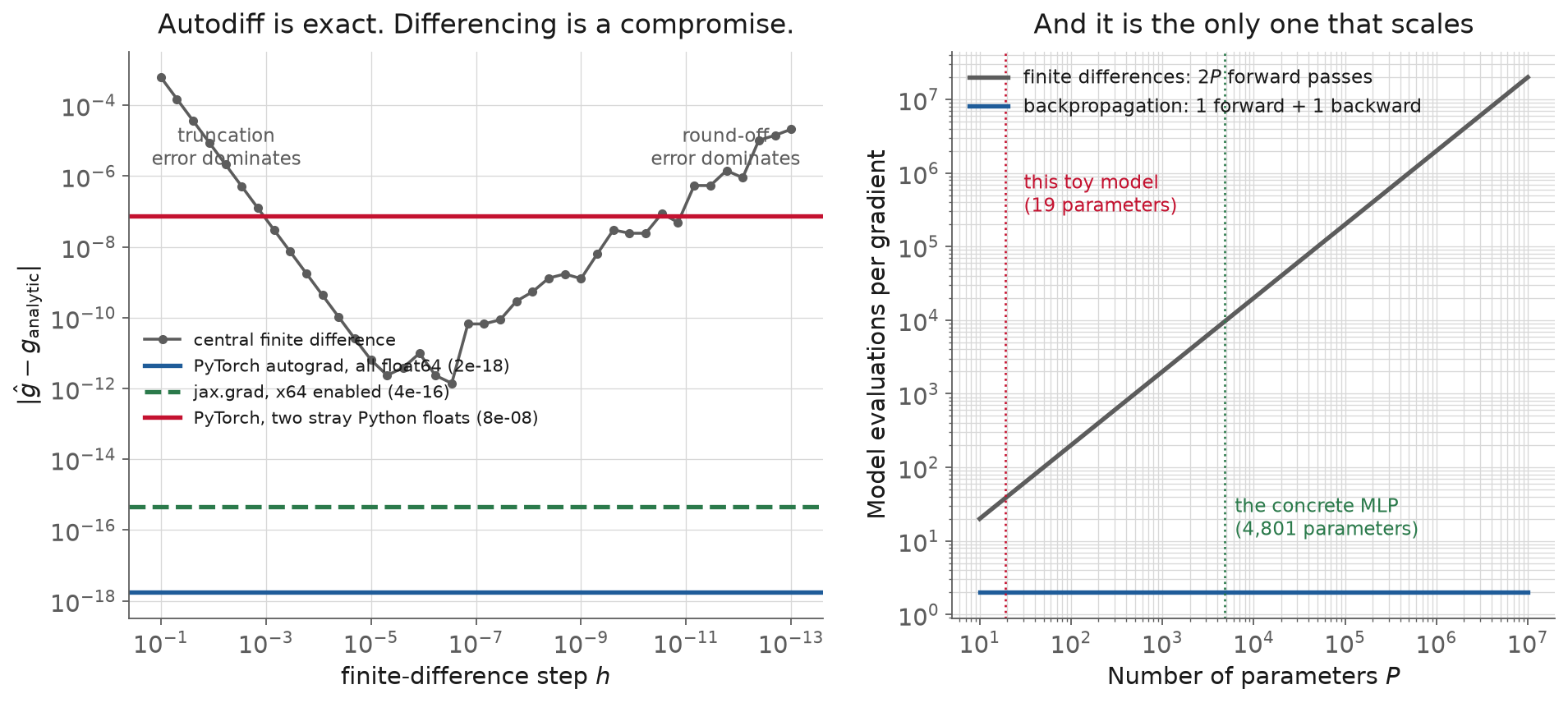
Fig. 66 Left: the same gradient computed four ways. The V is the classic trade between truncation and round-off; its best point, 1.4 × 10⁻¹², is four orders of magnitude worse than autodiff and requires knowing the right step size in advance. The red line is what one careless dtype costs, which the section on dtypes below explains. Right: why nobody uses finite differences for training.#
The measured numbers: PyTorch’s gradient differs from the hand-derived one by 1.7 × 10⁻¹⁸, JAX’s by 4.4 × 10⁻¹⁶, and the two agree with each other to 4.4 × 10⁻¹⁶, which is float64 epsilon. The best central difference, over forty step sizes, manages 1.4 × 10⁻¹² at h = 3 × 10⁻⁷, and you only know that was the best step because the exact answer was available to compare against, which in a real problem it is not. Finite differences keep one job in practice: checking an autodiff gradient you do not trust, at a handful of points.
PyTorch and JAX, two designs for the same mathematics#
The mathematics above is framework-independent. The two frameworks this session uses express it in opposite ways, and the contrast explains rules you would otherwise have to memorize. PyTorch records what your code does to tensors and differentiates the recording. JAX transforms the function you wrote into a new function that returns the derivative. Both produce the same numbers, to float64 epsilon, as the figure above shows.
PyTorch records a tape#
When a tensor has requires_grad=True, every operation on it appends a node to a graph, and
each node keeps a reference to whatever its backward rule will need. The
PyTorch autograd notes describe it as
a directed acyclic graph “whose leaves are the input tensors”, and state that “the graph is
recreated from scratch at every iteration”. This is called define-by-run. The graph is
whatever your Python code did on this call, so ordinary if statements and loops work unchanged,
and a different input can produce a different graph.
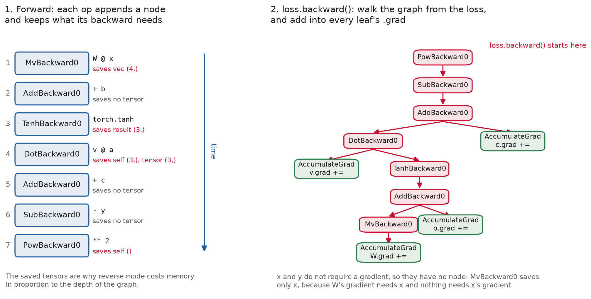
Fig. 67 The tape PyTorch actually recorded for the network above, read from loss.grad_fn. Left: the
seven nodes in the order the forward pass created them, and the tensors each one saved. Right:
the graph backward() walks. It ends in AccumulateGrad nodes, which add into .grad rather
than overwrite it. x and y get no nodes, because nothing asked for their gradient.#
The figure is drawn from a real loss.grad_fn, not a schematic. TanhBackward0 saves its own
output, because the derivative of tanh is \(1 - a^2\) and needs \(a\). MvBackward0 saves x,
which \(\partial L / \partial W = (\partial L / \partial z)\, x^\top\) needs. The additions save nothing, because their local
derivative is 1. Every saved tensor stays in memory until the backward pass has used it, which
is why training a model takes several times the memory of running it.
The tape ends in AccumulateGrad nodes, and those add into each parameter’s .grad
attribute. They do not overwrite it. Call backward() twice without clearing, and W.grad holds
exactly twice the gradient; the demo measures a ratio of 2.0. That is why the loop needs
optimizer.zero_grad():
loss = loss_fn(model(x), y)
optimizer.zero_grad()     # .grad += is the semantics, so you must clear it first
loss.backward()           # walks the tape, adds into every .grad
optimizer.step()          # reads .grad, updates the parameters
Accumulation is a deliberate choice with a real use. It lets you split a batch too large for
memory into micro-batches, call backward() on each, and step once on the sum, a technique
called gradient accumulation. The API is designed for that case, and the common case pays
for it with an extra line that is easy to forget. The section of stories below measures what
forgetting it costs.
Switching the tape off#
The tape has a cost that is easy to miss, because nothing about it shows in the code. To run the
backward pass, PyTorch must keep every intermediate value the forward pass produced, so each
recorded operation holds its inputs in memory until backward() consumes them or the last
reference to the graph disappears. During training that is the price of the gradient. Much of
what a training script does, though, never calls backward() at all, and there the stored graph
is pure overhead.
Measured on this laptop’s GPU, one forward pass of a two-layer MLP with 1,024 hidden units over a
batch of 8,192 rows leaves 67 MB held by the graph. The same pass inside torch.no_grad()
leaves 0.03 MB, the output alone, because intermediates are freed as soon as the next layer has
used them. The session’s 64-unit model on 1,030 rows holds 0.8 MB, which is why nobody notices
on a small problem.
The graph also lives as long as anything refers to it, which turns a harmless-looking line into
a leak. A validation loop that sums total += loss keeps a reference to every batch’s loss
tensor, and each of those keeps its whole graph alive. Over 50 batches of the 1,024-unit model
that held 478 MB, growing by about 10 MB per batch until the job runs out of memory
partway through an epoch. Writing total += loss.item() converts each loss to a Python float
and releases the graph, leaving 8 MB held, which is the last batch’s graph still bound to the
name loss. Running the loop inside no_grad() leaves nothing.
There are three situations where you want the tape off, and each has its own switch. The first
is evaluation, testing and serving, where no gradient is coming: wrap the pass in
with torch.no_grad():, or in torch.inference_mode(), a stricter and slightly faster variant
whose outputs can never re-enter a graph. The second is updating parameters by hand. Writing
W -= lr * W.grad raises a leaf Variable that requires grad is being used in an in-place
operation, and if it were allowed, the update would be recorded as part of the model. The update
goes inside torch.no_grad(), which is exactly what optimizer.step() does internally. The third
is blocking part of the model on purpose. A frozen pretrained layer gets
p.requires_grad_(False) on its parameters, and a value the loss should chase without moving,
such as a target computed by the model itself, gets .detach().
model.eval() is a different switch, and the two are easy to confuse. It changes layers whose
behavior differs between training and inference, dropout and batch normalization in particular,
and it has no effect on the tape. An evaluation pass needs both: eval() so the layers behave
as they will in deployment, and no_grad() so nothing is recorded. Forgetting eval() is a
classic source of a validation score that differs from the test score another script computes,
and model.train() switches the layers back before the next epoch.
JAX needs almost none of this. Nothing is recorded unless the function is called under
jax.grad, so an evaluation pass is an ordinary function call, and parameters are immutable
arrays, so an update builds new ones rather than editing old ones in place. The one case left is
the third: jax.lax.stop_gradient(x) passes x through unchanged while telling grad to treat
it as a constant.
JAX transforms functions#
JAX takes the opposite route. jax.grad(f) does not compute a gradient. It returns a new
function that computes one. There is no tape, no mutable .grad, and consequently nothing to
zero:
import jax, jax.numpy as jnp

def loss(params, x, y):
    a = jnp.tanh(params["W"] @ x + params["b"])
    return (params["v"] @ a + params["c"] - y) ** 2

grads = jax.grad(loss)(params, x, y)     # same structure as params, no state touched
To build that new function, JAX traces the original. It calls loss once with placeholder
values that record each operation, and writes the result down in a small intermediate language
called a jaxpr. The jaxpr documentation is short
and worth reading. jax.make_jaxpr prints it, and for the loss above it is seven equations, one
per operation in the forward pass:
{ lambda ; a:f64[3,4] b:f64[3] c:f64[] d:f64[3] e:f64[4] f:f64[]. let
    g:f64[3] = dot_general[...] a e
    h:f64[3] = add g b
    i:f64[3] = tanh h
    j:f64[] = dot_general[...] d i
    k:f64[] = add j c
    l:f64[] = sub k f
    m:f64[] = integer_pow[y=2] l
  in (m,) }
The same seven steps appear in PyTorch’s tape. The difference is what happens next. jax.grad
transforms this program into a longer one, sixteen equations, that computes the forward pass and
the backward pass together; you can print that one too. The tanh derivative shows up as an
explicit 1 - i multiplied through. The gradient is itself a program, so it can be transformed
again: jax.grad(jax.grad(f)) differentiates twice, and jax.jit compiles the result through
XLA, the compiler JAX uses to generate code for CPUs, GPUs and TPUs.
Tracing has a price that the tape does not. The jaxpr records one path through your code, so a
Python if that depends on the value of an array cannot be traced. It needs jax.lax.cond,
and a loop whose length depends on data needs jax.lax.while_loop. The function must also be
pure. It may not modify its inputs, and any side effect, such as a print or an append to a
global list, runs once at trace time and then never again. The
key concepts page lays out the rules.
JAX batches with vmap and compiles with jit#
PyTorch asks you to honor a batch dimension in every module you write. JAX takes another route:
write the function for one example and let vmap add the batch axis.
def predict_one(params, x):                    # no batch dimension anywhere
    return params["v"] @ jnp.tanh(params["W"] @ x + params["b"]) + params["c"]

predict_batch = jax.vmap(predict_one, in_axes=(None, 0))   # params shared, x batched
Seeing this once is useful even if you never write JAX, because it shows what the batch
dimension is: an axis you are mapping over, which the model itself does not need to know about.
In the demo, vmap agrees with an explicit Python loop over the same 256 examples to 2.2 × 10⁻¹⁵,
and it is faster, because it becomes one batched kernel rather than 256 small ones.
The same framing explains jax.jit, which compiles a function through XLA and fuses what it
can into single kernels. What that is worth depends entirely on what you give it, and the demo
measures three cases rather than quoting one:
workload |
eager |
jit |
|
|---|---|---|---|
one 512×512 matmul plus |
2.8 ms |
3.6 ms |
0.8× |
a chain of elementwise ops on 2M floats |
16.8 ms |
14.6 ms |
1.2× |
a 10-step iterative update via |
83.3 ms |
30.3 ms |
2.8× |
Compiling a single large matrix multiply gained nothing here: there is nothing to fuse, the eager path was already one call into an optimized BLAS kernel, and the compiled version adds dispatch. Compiling a loop of many small operations is worth 2.8×, because that is exactly what fusion removes. These are wall-clock timings on a shared laptop, and a later rerun of the same script put the matmul at 1.2× and the loop at 4.3×, so trust the ordering rather than the magnitudes. Compilation pays when there are many small operations to collapse. The same argument decides whether a GPU pays, as the section on devices shows.
PyTorch has adopted both ideas. torch.func provides grad, vmap, jvp and vjp as
function transforms in the JAX style, and torch.compile compiles a model into fused kernels.
The difference between the two frameworks is now mostly one of defaults. PyTorch starts eager and
stateful and lets you opt into transforms. JAX starts functional and compiled and asks you to
give up mutation to get there.
Side by side#
concept |
PyTorch |
JAX |
|---|---|---|
array |
|
|
default float |
float32 |
float32 |
float64 |
on request: |
only after |
gradient |
|
|
state |
inside |
explicit: parameters and optimizer state are values you pass in and get back |
turn off gradients |
|
do not differentiate it, or |
train or eval behavior |
|
an explicit argument, such as |
batch |
a leading dimension in every module |
|
compile |
|
|
randomness |
a global generator, |
explicit keys, |
optimizers |
|
the optax library |
Tensors, shapes, and dtypes#
A PyTorch tensor is a NumPy array with three extra properties. It knows what device it
lives on, it can record the operations performed on it so they can be differentiated, and its
default dtype is not the one NumPy would have picked. A JAX array has the first and third
properties. It is differentiable because the function using it is transformed, and it is
immutable: x[0] = 1.0 raises a TypeError, and x = x.at[0].set(1.0) returns a new array
instead.
Definition: tensor
A tensor is an n-dimensional array with a shape, a dtype and a device. In PyTorch it can also record the operations applied to it, so gradients can be computed through them.
Shapes and broadcasting work as they do in NumPy in both libraries, and the same mental model
applies. An operation between a (N, 1) and a (N,) array broadcasts into (N, N), which is
almost never what you meant. It raises no error, and the section of stories below shows what it
does to a model. Views and copies also behave as in NumPy in PyTorch: reshape may return a view
sharing storage, clone does not, and mutating a view mutates the original. The autograd engine
tracks this, so an in-place operation on a tensor needed for the backward pass raises a helpful
error, one of the few places PyTorch does complain.
The batch dimension comes first. Every built-in module in PyTorch expects input shaped
(N, ...), where N indexes examples: (N, features) for a multilayer perceptron (MLP),
(N, channels, height, width) for a 2D convolution, and (N, channels, time) for a 1D
convolution over a sensor window. The convention makes the batch the outermost, contiguous axis,
so a batch is one slab of memory that can be shipped to an accelerator in a single transfer.
Shape errors are the most common crash in a first training script, and they read as a sentence
once you know which matrix is which. Suppose the model is
nn.Sequential(nn.Linear(8, 64), nn.ReLU(), nn.Linear(64, 1)) and a batch of 32 concrete samples,
each with 8 features, reaches the last layer without passing through the first, perhaps because
the model was assembled by hand and a layer was skipped. PyTorch reports
mat1 and mat2 shapes cannot be multiplied (32x8 and 64x1). The first matrix is always your
input: 32 rows, 8 features. The second is the layer’s weight, transposed, because nn.Linear(64, 1)
stores its weight as (1, 64) and computes x @ W.T, so it reads 64x1 and says this layer
expects 64 input features. A matrix product needs the inner dimensions to agree, and 8 is not
64. The fix is never to reshape the input until the numbers match. It is to find why this layer
received 8 features when it was built for 64: a skipped layer, as here, or an in_features that no
longer matches the data after a column was added or dropped. Choosing a batch size that differs
from every layer width, as 32 does here, makes these messages far easier to read, because no two
numbers in them coincide.
JAX has one more behavior to watch for. Indexing out of bounds does not raise, because
raising from compiled code on an accelerator is expensive. A read is clamped to the last valid
element, so jnp.arange(3.0)[10] returns 2.0, and an out-of-bounds write is silently dropped.
The JAX sharp bits page
lists this with the others, and it is worth reading before you write any JAX.
The dtype trap, measured#
torch.tensor(3.14) gives you a float32 tensor, and torch.tensor(np.float64(3.14)) gives
you float64. NumPy defaults to float64 and PyTorch defaults to float32. When a float32 tensor
meets a float64 one, the result is float64, so every dtype you inspect downstream of the
mistake reads float64 and looks fine.
None of this means PyTorch is weak at double precision. It supports float64 fully on the CPU and
on CUDA GPUs: pass dtype=torch.float64, call .double() on a tensor or a model, or call
torch.set_default_dtype(torch.float64) once at the start of a program so that every new
floating-point tensor is float64. The exception is Apple’s MPS backend, which has no float64 at
all and raises an error if you move a float64 tensor onto it. Elsewhere float64 is available;
the problem is that float32 is the default.
This happened while these notes were written, and it is the first of this session’s stories. The autodiff figure above was meant to show that PyTorch and JAX both agree with a hand-derived gradient to machine precision. JAX did. PyTorch disagreed at 7.5 × 10⁻⁸, eight orders of magnitude worse than it should be. Every tensor in the calculation reported float64, and the code had been checked. It looked like a genuine difference between the two libraries.
It was not. Two scalars in the setup were Python floats, 1.234 and the output of a bare
rng.normal() call, and torch.tensor stored both as float32. The relative error that produced
was 1.25 × 10⁻⁷, which is float32 epsilon to two figures. Declare those two scalars as
float64 and PyTorch’s gradient matches the analytic one to 1.7 × 10⁻¹⁸. The size of the error
identified the cause: a discrepancy near 10⁻⁷ is float32’s fingerprint.
JAX makes the same mistake in the opposite direction, and more quietly. By default JAX has
64-bit types switched off, so every float array is float32, including one built from a
float64 NumPy array. jnp.asarray(np.ones(3)) returns float32 with no warning at all. JAX warns
only when you explicitly ask for dtype=jnp.float64, and even then it truncates. Setting
jax.config.update("jax_enable_x64", True) at the start of the program turns 64-bit types on.
The autodiff figure’s JAX line agrees to 4.4 × 10⁻¹⁶ only because the script does that first.
What a practitioner should take from this
Set the dtype explicitly at every boundary where data enters a tensor, and do not rely on the
default. torch.tensor(x, dtype=torch.float32) is four extra words that document an intent. In
JAX, decide on jax_enable_x64 once, at the top of the program, before any array is created.
This is the same bug as in Lecture 7. A quantity crossed an
interface, its type was silently converted, nothing raised, and every diagnostic downstream
reported the promoted type rather than the one that lost the information. Checking
tensor.dtype after the fact would not have found this. Checking it at the boundary would have.
Four models that looked fine#
The dtype story has a pattern that the rest of this section repeats. The code runs, a number
comes out that looks plausible, and nothing raises. Only a comparison against something you
trust, such as an analytic gradient, a trivial baseline, or an honest split, shows that the
number is wrong. Each story below gives what the run looked like, why it looked fine, what the
cause was, and what the number became once it was fixed. All of them use the same dataset, the
same small network, and the same validation fold. The notebook
l11-four-models.ipynb reruns all four from the code that produced these
numbers, with a cell for each that exposes the cause, so you can take any of them apart yourself.
Look at the rows before you model them#
The dataset is concrete compressive strength, introduced in Lecture 9: 1,030 test results from I-Cheng Yeh’s 1998 study, with eight inputs (cement, blast-furnace slag, fly ash, water, superplasticizer, coarse and fine aggregate, and age in days). The target is the result of a crush test that destroys the specimen and is usually run after 28 days of curing, which is exactly the trade a surrogate model exists to make. It is also small and tabular, which is where the received wisdom says deep learning loses.
Before modeling, apply Lecture 9’s question: are these rows exchangeable? They are not, and nothing in the file announces it. Group the rows by their seven mix components, ignoring age, and the 1,030 rows collapse into 428 distinct mixes. Of those, 182 were tested at more than one age, and those multi-age mixes account for 76% of all rows. The same batch of concrete appears at 3, 7, 28 and 90 days, as separate rows. The file also contains 25 exact duplicate rows, identical in all nine columns.
How much scatter is even there?
The dataset contains just enough replication to show there is irreducible noise, and nowhere near enough to measure it well. Eight settings have the same mix and the same age measured twice with different results, and those pairs differ by 0.89, 1.28, 1.48, 1.68, 1.97, 2.86, 3.44 and 6.60 MPa. Treating them as duplicate measurements gives a repeatability standard deviation of about 2.2 MPa, on eight degrees of freedom.
Take that as an order of magnitude. A model reporting an RMSE near 2 MPa on this dataset would be claiming to predict the test better than the test can reproduce itself.
One more group was excluded from that estimate: four rows with identical features at 7 days, three of which report exactly 55.895819 MPa and the fourth 22.897498. That is one bad number, and averaging it into a repeatability estimate would have tripled the estimate.
Unless a story says otherwise, it reports validation RMSE on the first fold of a GroupKFold split by mix, where
predicting the training mean scores 17.9 MPa and the working network scores 5.5 MPa.
The loss went down and the model learned a constant#
How it looked. The loop trained for 120 epochs without an error. The training loss fell steadily, which is what everyone checks first. The validation RMSE was 17.7 MPa.
Why it looked fine. 17.7 MPa is an unremarkable number for a first attempt, and without a baseline nothing marks it as a failure. The baseline says otherwise. Predicting the training mean for every row scores 17.9, so the network was 1% better than no model at all. The standard deviation of its predictions across the validation mixes was 0.26 MPa, where the true strengths spread over tens of MPa. The network had learned to output a constant.
The cause. The model returns predictions of shape (64, 1). The targets were stored as
(64,). nn.MSELoss subtracts one from the other, and broadcasting turns that into a (64, 64)
matrix of every prediction minus every target. The mean of that matrix is minimized by predicting
the batch mean for every row, so that is what the network learned, and the loss really did go
down. PyTorch emitted a warning, “Using a target size (torch.Size([64])) that is different to the
input size (torch.Size([64, 1])). This will likely lead to incorrect results”, once per batch,
1,560 times in all. A Jupyter notebook shows a repeated warning once, at the top of a long cell.
Fixed. Give the target the model’s shape, y[:, None], or squeeze the prediction. Validation
RMSE is 5.5 MPa, and the predictions spread by 16.2 MPa, matching the data.
What a practitioner should take from this
Assert the shapes at the loss: assert pred.shape == target.shape costs one line and catches this
class of bug in the first batch. Compare every model with the predict-the-mean baseline, and look
at the spread of the predictions, not only their error. A model whose predictions barely vary has
not learned the inputs, whatever its loss curve says.
The tree that won on a leaky split#
How it looked. A careful comparison, five seeds by five folds, of gradient boosting against
the PyTorch MLP under an ordinary random KFold. Gradient boosting scored 4.44 MPa and the
MLP 4.87. The tree won by 0.43 ± 0.09 MPa, nearly five standard errors, and it matched the
received wisdom that trees beat networks on small tabular data. Both numbers are within about
2.5 MPa of the test’s own repeatability, which looks like excellent work.
Why it looked fine. Everything about the protocol was right except the split, and the split is invisible in the output.
The cause. A random k-fold puts rows from the same mix on both sides of the split, so the
model is asked to predict a curing curve it has already seen most of. This is the airfoil
frequency sweep from Lecture 9 in a different material, and the 25 duplicate rows make it worse.
Under a GroupKFold on the mix, gradient boosting scores 6.25 and the MLP 6.48. The
gap is 0.23 ± 0.18 MPa, less than two standard errors. On this dataset, honestly evaluated, the
two models tie.
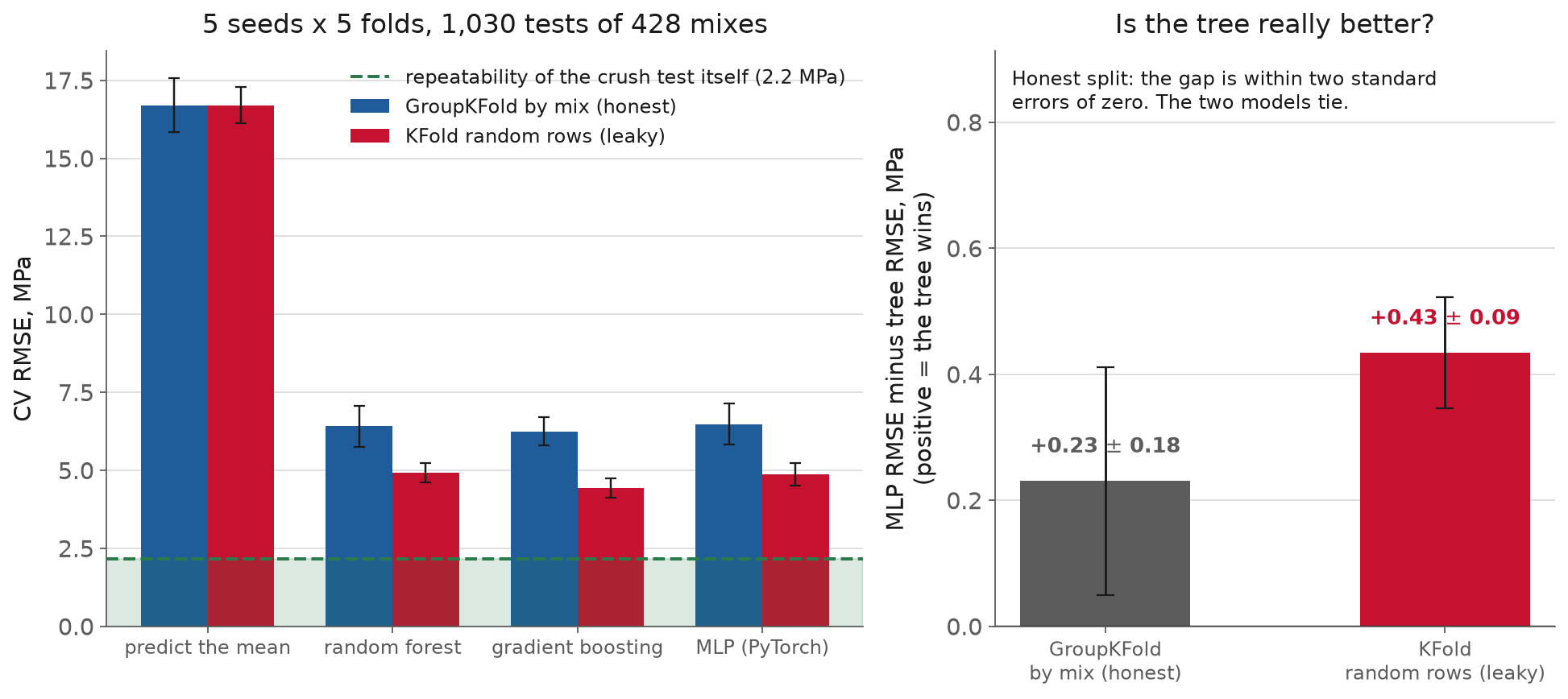
Fig. 68 Five random seeds by five folds, so 25 measurements per bar. Everything gets better under the random split; the question is which model gets better faster.#
Both models get worse when the leak is closed, which is expected. What is less expected is that the tree gets worse faster: it gains 1.81 MPa from the leaky split against the MLP’s 1.61. Gradient boosting exploits a near-duplicate row better than a small MLP does, so part of “trees beat nets on small tabular data” was, on this dataset, a statement about the split.
The classic leak, fitting the StandardScaler on every row before splitting, was measured on the
same folds as well: 6.27 MPa with the scaler fitted on the training rows only, 6.23 with it
fitted on all rows, a difference of −0.04 ± 0.06 over fifteen runs. Here that leak costs nothing
measurable, because the scaler learns eight means and eight standard deviations, and the
validation rows barely move them. It is still a bug, and on a smaller or drifting dataset it will
not be free. The leak that changed this comparison was the split.
That is a narrower claim than it may sound. One dataset with 1,030 rows is not a refutation of anything. Grinsztajn, Oyallon and Varoquaux benchmarked 45 datasets with 20,000 compute hours of hyperparameter search per learner and concluded that “tree-based models remain state-of-the-art on medium-sized data (~10K samples).” They identify three reasons rooted in inductive bias: neural networks struggle to be “robust to uninformative features,” to “preserve the orientation of the data,” and to “easily learn irregular functions.” Nothing here contradicts that. The concrete measurement shows something narrower and still useful: before you attribute a model-family gap to inductive bias, check that it is not a split artefact.
What a practitioner should take from this
Run the comparison on the honest split first. A model-selection conclusion drawn on a leaky split can change when the leak is closed, because model families exploit leaks by different amounts.
And a single seed is not a result. The first version of this comparison ran one seed and showed the MLP beating gradient boosting under the grouped split. Five seeds show a tie. The spread across seeds on this problem is comparable to the difference between model families, so report the mean and spread over at least five seeds, or do not report a comparison.
The loop that forgot zero_grad()#
How it looked. The loop ran, the loss printed every epoch, and the validation RMSE moved around between about 10 and 17 MPa for most of the run, below the 17.9 baseline. A curve like that reads as “noisy, needs a smaller learning rate”. It does not read as a bug.
Why it looked fine. A model that beats the baseline and whose loss is not NaN looks like a model that is learning. The oscillation looks like a hyperparameter problem, so the natural response is to tune, which hides the cause further.
The cause. The optimizer.zero_grad() line was missing, so .grad accumulated across steps.
The gradient used at step k is the sum of the gradients from every step before it, so the
effective step size grows through the run and the model wanders. After 120 epochs this run
finished at 23.2 MPa, worse than predicting the mean, but the number it ends at depends on
where you stop. Several epochs earlier it sat near 12.
Fixed. Restore the line. The same code, seed and fold score 5.5 MPa, and the validation curve settles instead of wandering. The left panel of the figure below shows both runs.
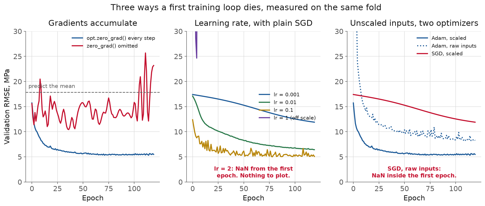
Fig. 69 The same fold, the same architecture, one thing changed at a time.#
What a practitioner should take from this
Before tuning a learning rate, read the loop against the five-line template in the next section
and log the gradient norm for a few steps. Without zero_grad() the norm grows every step, from
0.13 to 0.93 over the first eight in the notebook, while a correct loop’s stays between 0.12
and 0.16. When the validation curve oscillates and the gradient norm climbs in a straight line,
fix the loop before touching the learning rate.
Adam on raw inputs#
How it looked. The inputs went into the network unscaled, and training with Adam converged smoothly to a validation RMSE of about 8 MPa, less than half the baseline. There was no NaN, no warning, and a loss curve that looks like the textbook shape.
Why it looked fine. 8 MPa is a respectable number, and the usual warning about unscaled inputs is that training diverges. This run did not diverge, so the warning did not seem to apply.
The cause. The concrete features run from coarse aggregate, averaging about 970 kg/m³, to superplasticizer, averaging about 6, a factor of more than 150. With SGD that produces NaN within the first epoch, the loud failure the warning describes. With Adam it does not diverge at all: it trains to 8.3 MPa instead of 5.5, a model that works, is half again as bad as it should be, and gives no indication that anything is wrong. The section on Adam below explains why: Adam rescales each parameter’s step by the size of its own gradient, which absorbs the scaling problem that makes SGD explode, but it cannot fully undo it.
Fixed. Fit a StandardScaler on the training rows and apply it to both splits. Adam reaches
5.5 MPa.
What a practitioner should take from this
Adam’s per-parameter step size makes it forgiving, and forgiveness hides bugs. SGD reports a scaling bug by exploding; Adam absorbs the same bug and hands you a mediocre model. If your Adam-trained network is merely disappointing and you have never scaled its inputs, scale them before you touch the architecture.
Scale on the training split only, with the fitted transform applied to validation and test, exactly as in Lecture 7. The habit does not change because the model is now a neural network, even on a dataset where the leak happens to be small.
The anatomy of a training loop#
With the gradient understood, the loop is short. It has four objects and five lines, and two of
the stories above were one wrong line in it: the target’s shape and the missing zero_grad().
The loop runs on mini-batches, as Lecture 9 introduced them. Each pass through the inner loop computes the gradient on a small random slice of the rows, 64 here, which is a noisy estimate of the full gradient, and takes one optimizer step with it. One pass over every row is an epoch, so a 120-epoch run on 824 training rows takes 120 × 13 = 1,560 steps. That is where the 1,560 warnings in the first story came from: one per step.
A Dataset answers two questions, __len__ and __getitem__, and a DataLoader wraps
one to produce shuffled batches, optionally in parallel worker processes. For a table that fits
in memory, as this session’s does, you can skip both and index tensors directly. The DataLoader
earns its place when examples must be read or decoded from disk, and num_workers matters when
that decoding is the bottleneck rather than the arithmetic.
An nn.Module holds parameters and defines forward. A loss function reduces
predictions and targets to a scalar, as Lecture 9 defined it: MSELoss for regression when large
errors should hurt quadratically, L1Loss when they should not, and CrossEntropyLoss for
classification. CrossEntropyLoss expects raw logits rather than probabilities and applies the
softmax itself, a detail that produces a lot of quietly mistrained classifiers.
An optimizer turns gradients into parameter updates. The next subsection opens up the one this session uses.
for epoch in range(n_epochs):
    model.train()
    for xb, yb in loader:
        xb, yb = xb.to(device), yb.to(device)
        loss = loss_fn(model(xb), yb)   # forward
        optimizer.zero_grad()           # clear the accumulator
        loss.backward()                 # backward
        optimizer.step()                # update
The JAX version of the same loop makes every piece of state explicit. The parameters are a dictionary, the optimizer comes from optax, its state is a value you pass in and get back, and the shuffle takes an explicit random key:
optimizer = optax.adam(1e-3)
opt_state = optimizer.init(params)

@jax.jit
def step(params, opt_state, xb, yb):
    loss, grads = jax.value_and_grad(loss_fn)(params, xb, yb)
    updates, opt_state = optimizer.update(grads, opt_state, params)
    return optax.apply_updates(params, updates), opt_state, loss

for epoch in range(n_epochs):
    key, sub = jax.random.split(key)
    perm = jax.random.permutation(sub, n)
    for i in range(0, n, 64):
        idx = perm[i:i + 64]
        params, opt_state, loss = step(params, opt_state, X[idx], y[idx])
There is no zero_grad, because value_and_grad returns fresh gradients each call, and there is
no .to(device), because JAX places arrays on the default device itself. Both loops train the
same 8-64-64-1 network with the same initialization scheme on the same fold. Over five seeds the
PyTorch loop scores 5.70 ± 0.29 MPa and the JAX loop 5.66 ± 0.24, the same model to within
the seed-to-seed spread.
Adam, and what its parameters do#
Lecture 9 introduced Adam as stochastic gradient descent with two running averages. Here are the equations, because each hyperparameter is visible in them. At step \(t\), with gradient \(g_t\), learning rate \(\eta\), and running averages \(m_t\) of the gradient and \(v_t\) of its square (this \(v\) follows the paper’s notation and is unrelated to the network’s output weight above):
Definition: Adam
Adam updates each parameter by a running average of its gradient (momentum), divided by the square root of a running average of its squared gradient, so every parameter gets its own step size.
Each piece has a job, and the figures below show each one on a small problem where you can see it: the long, narrow bowl \(L = (\theta_1^2 + 40\,\theta_2^2)/2\), which is steep in one direction and shallow in the other, like a network whose inputs were never scaled.
\(\eta\), the learning rate, sets the size of every step. Because the update divides the gradient by its own magnitude, a step of Adam is about \(\eta\) long in each coordinate, whatever the gradient’s size.
\(\beta_1\), momentum, averages the gradient over roughly \(1/(1-\beta_1)\) steps, ten at the default of 0.9. It smooths mini-batch noise and carries the iterate along a consistent direction.
\(\beta_2\) averages the squared gradient over roughly \(1/(1-\beta_2)\) steps, a thousand at the default of 0.999. It sets how quickly the per-parameter step size adapts.
\(\epsilon\) keeps the division finite. At its default of \(10^{-8}\) it is negligible; made large, it turns Adam back into momentum SGD for any parameter whose gradient is smaller than \(\epsilon\).
Bias correction, the division by \(1 - \beta^t\), exists because both averages start at zero. Without it, the first step would be about 3.2 times the learning rate rather than equal to it, because \(\sqrt{v_1}\) is only \(\sqrt{0.001}\) of the gradient’s size.
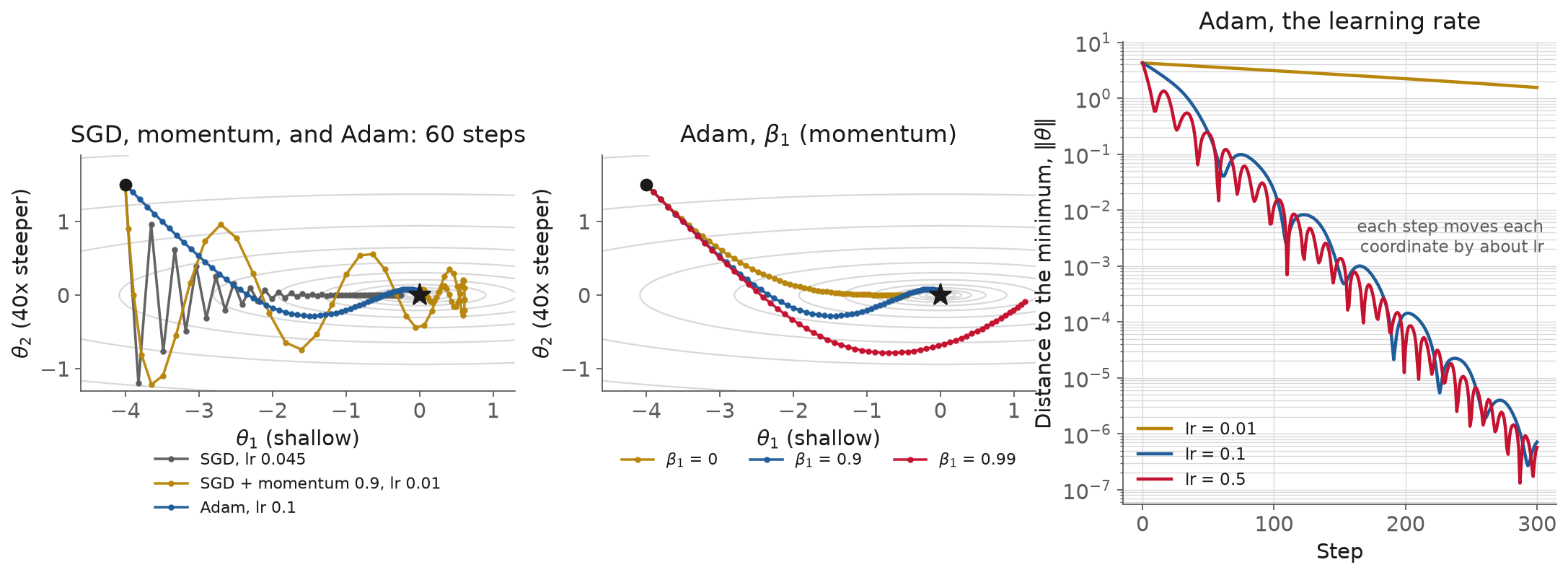
Fig. 70 Adam on the bowl \(L = (\theta_1^2 + 40\theta_2^2)/2\), from the same start. Left: 60 steps of SGD,
SGD with momentum, and Adam. Middle: momentum \(\beta_1\); at 0.99 it overshoots and the loss
after 100 steps is 5.3 against 0.0011 at the default. Right: the learning rate; after 300
steps, 0.01 is still 1.6 units from the minimum while 0.1 has converged to 7 × 10⁻⁷. The update
code matches torch.optim.Adam to 4.4 × 10⁻¹⁶ and optax.adam to 2.2 × 10⁻¹⁶.#
The left panel shows the property that matters most. Plain SGD’s first step is 2.7 units along the steep coordinate and 0.18 along the shallow one, so it zig-zags across the valley. Adam’s first step is 0.1, the learning rate, in both coordinates. It is invariant to a rescaling of each parameter, which the original paper states as “invariant to diagonal rescaling of the gradients”. That property is why Adam survived the unscaled concrete inputs where SGD produced NaN, and it is also why Adam hid the bug.
The invariance is per coordinate, and only per coordinate. Rotate the same bowl by 45°, so the narrow direction no longer lines up with a parameter axis, and Adam’s loss after 100 steps goes from 0.0011 to 1.1. Adam can rescale each parameter separately, but it cannot correct for two parameters that are coupled. Scaling the inputs aligns the problem with the axes in a way Adam cannot do for itself.
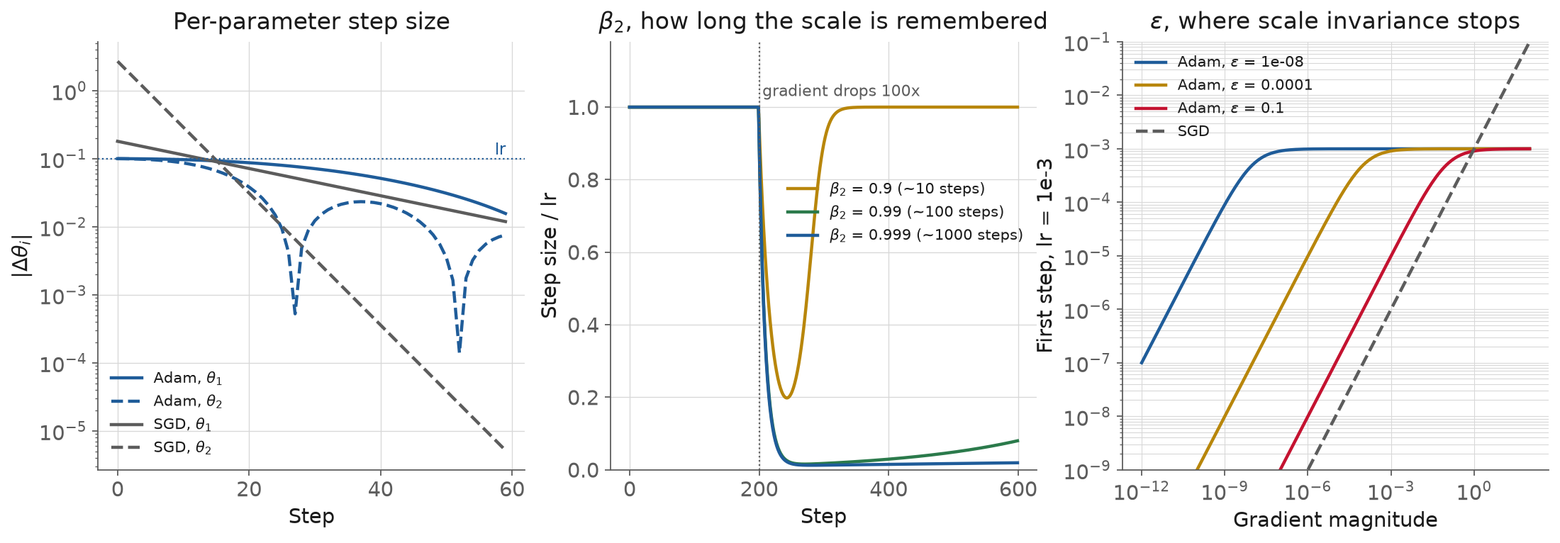
Fig. 71 What \(\beta_2\) and \(\epsilon\) do. Left: Adam’s steps start equal in each coordinate; SGD’s differ by the ratio of the gradients. Middle: when the gradient drops 100-fold, \(\beta_2 = 0.999\) remembers the old, large gradients and the step collapses about sixty-fold for hundreds of steps, while \(\beta_2 = 0.9\) dips five-fold and recovers within about a hundred. Right: a large \(\epsilon\) makes the first step proportional to the gradient, like SGD, once the gradient is smaller than \(\epsilon\).#
AdamW fixes a subtle problem with regularization. Adding an L2 penalty to the loss is the same as shrinking the weights at each step for plain SGD, but not for Adam, because Adam divides the penalty’s gradient by \(\sqrt{\hat{v}}\) like every other gradient. Loshchilov and Hutter put it directly: “L2 regularization and weight decay regularization are equivalent for standard stochastic gradient descent … not the case for adaptive gradient algorithms, such as Adam”. AdamW applies weight decay directly to the weights, outside the adaptive scaling.
The defaults differ between the frameworks in one place that matters when you port code.
PyTorch’s Adam and optax’s adam agree on \(\beta_1 = 0.9\), \(\beta_2 = 0.999\) and
\(\epsilon = 10^{-8}\); PyTorch defaults the learning rate to \(10^{-3}\) and optax requires you to
pass one. But torch.optim.AdamW defaults to a weight decay of 0.01 and optax.adamw to
0.0001, a factor of one hundred. A model ported from one to the other with default arguments
is regularized a hundred times more or less, and nothing will say so.
The learning rate#
The learning rate is the hyperparameter that most often decides whether a run works at all. The
middle panel of the pathology figure sweeps it for plain SGD. At 0.001 it is too small to
converge in the budget: 11.9 MPa after 120 epochs and still descending. At 0.01 it reaches 6.4,
at 0.1 it reaches 5.1, and at 2.0 it produces NaN from the first epoch onward. The failure at
2.0 is total rather than gradual: there is no partially diverged run to diagnose, just a column
of nan.
The boundary between those is fuzzier than the tidy version of this lesson admits. At
lr = 1.0 the outcome depends on the seed: across six seeds it produced nan in two and
diverged to between 91 and 1,235 MPa in the other four. A learning rate is not simply stable or
unstable. It is stable for this initialization, and a single run that survived is not evidence
that the next one will.
Devices, and when a GPU helps#
Moving a PyTorch model to a GPU is two lines: model.to(device) and x.to(device). The rules
are few. Model and data must be on the same device or you get a clear error, which is the good
case. Anything you print, plot or hand to NumPy must come back with .cpu(), and doing that inside
the training loop silently serializes the whole thing, because it forces the accelerator to
finish before the copy can start.
JAX places arrays on the default device automatically, the first GPU if one is visible, so there
is no .to() in the loop above. jax.devices() lists what it found, and jax.device_put moves
an array explicitly. Both frameworks share one trap. A GPU runs work asynchronously, so a call
returns as soon as the work is queued. Timing GPU code measures how fast you queued the work
unless you wait for it: torch.cuda.synchronize() in PyTorch, and x.block_until_ready() in JAX,
which the asynchronous dispatch page
explains.
A GPU is a throughput device with a large fixed cost per kernel launch. It makes wide operations cheaper per element, and does nothing for an operation too narrow to fill it. If your operation is narrow, the launch overhead dominates and the accelerator loses.
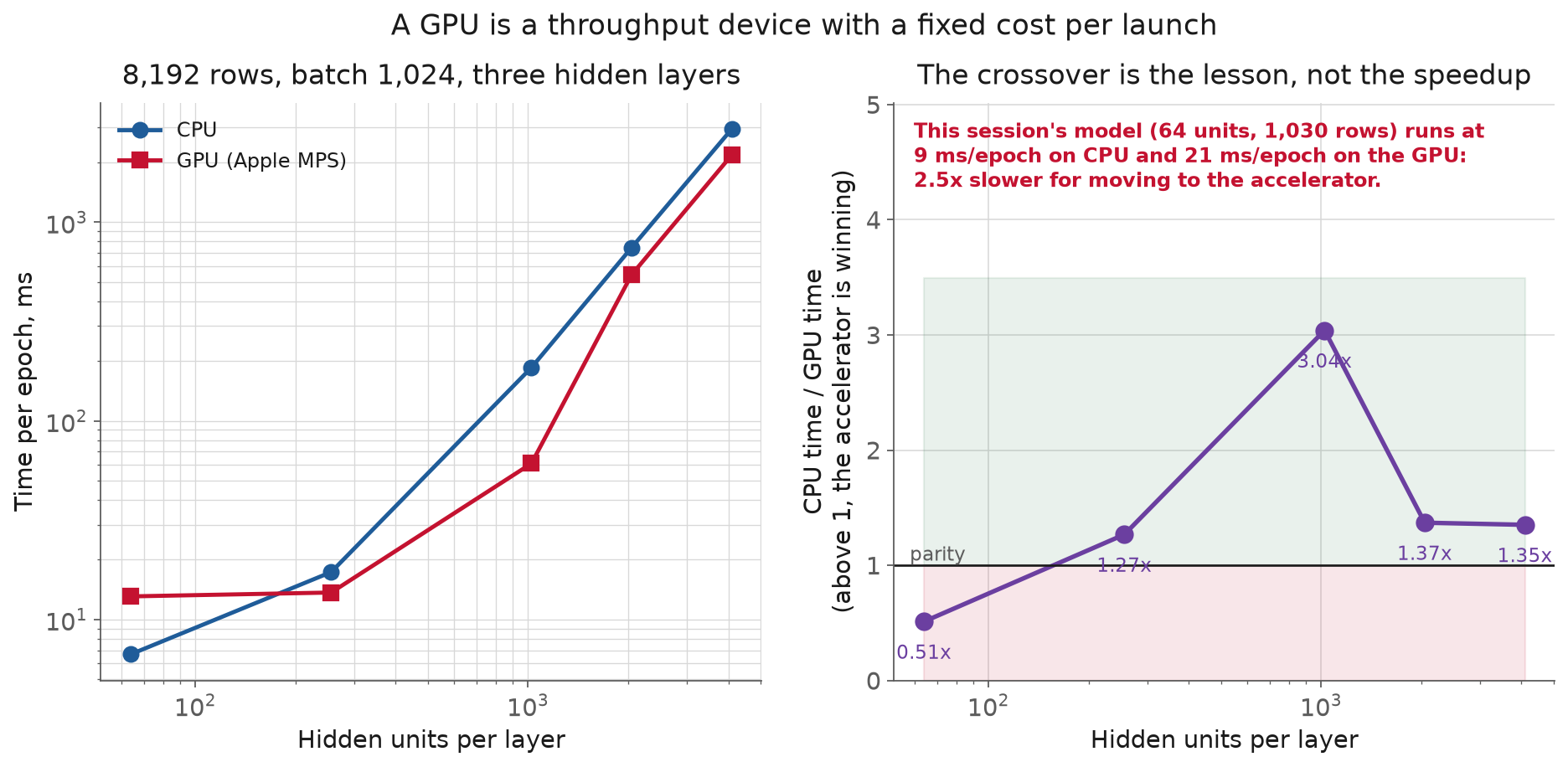
Fig. 72 Epoch time for a three-layer MLP on 8,192 synthetic rows, batch 1,024. Below roughly 200 hidden units the CPU wins outright; the accelerator only pays once there is enough arithmetic behind each launch. Measured on Apple MPS, because that is the accelerator this laptop has.#
This session’s actual model, an MLP with two hidden layers of 64 units trained on 1,030 rows, runs at 8.6 ms per epoch on the CPU and 21.1 ms on the GPU. Moving it to the accelerator makes it two and a half times slower. The crossover in the figure sits between 64 and 256 hidden units, and past it the accelerator wins by factors between 1.3 and 3 on this hardware.
Those timings are the least reproducible numbers in these notes. They are wall-clock measurements on a shared laptop, and an earlier run of the identical script reported 11.2 ms and 33.9 ms for the same two configurations, because something else was competing for the machine. The figures report the minimum over repeated trials rather than the mean, which is standard practice for microbenchmarks: interference can only make a measurement slower, so the minimum is the stable estimate. Expect the ratios to move by tens of percent on your hardware, and expect the crossing to be there.
A caveat about these numbers
These are Apple MPS measurements on a laptop, because that is the accelerator available where these figures were generated. A datacenter CUDA card has a much higher ceiling, and speedups of 10× to 50× on a large model are ordinary.
What transfers is the shape of the curve. There is a fixed cost per kernel launch on every accelerator, so the crossover exists on every accelerator; a bigger card moves it and raises the plateau. The practical consequence is the same either way: debug on CPU with a tiny subset, then launch the real run on the GPU. For a model the size of this session’s, the CPU is the correct choice.
Mixed precision is worth knowing about but not worth using yet. It runs the bulk of the
arithmetic in float16 or bfloat16 while keeping a float32 copy of the weights, roughly halving
memory and often doubling throughput on hardware with tensor cores. In PyTorch that is
torch.autocast, plus a GradScaler for float16, whose narrow exponent range lets small
gradients underflow to zero; the scaler multiplies the loss up before the backward pass and
divides the gradients down after. In JAX you choose the dtypes of the computation yourself.
Reach for it when a model does not fit or is too slow, not before.
Reproducibility and random seeds#
A deep learning run has more sources of randomness than a scikit-learn fit: parameter
initialization, batch shuffling, dropout masks, and on a GPU the non-deterministic reduction order
of some kernels. In PyTorch, seeding torch, NumPy and Python’s random covers the first three,
and torch.use_deterministic_algorithms(True) covers most of the fourth, at a speed cost.
JAX has no global random state at all. Every random function takes a key as an argument, and
you derive new keys with jax.random.split, as the shuffle in the JAX loop above does. Reusing a
key gives the same numbers again, which is a common first bug, and the
random numbers page explains why the design
is worth it: randomness that is an explicit value can be reproduced exactly, including inside
jit and vmap, and two parts of a program cannot silently share a generator.
In either framework, seeding makes a run reproducible. It does not make it representative. A single seeded run is one draw from a distribution, and the width of that distribution is a property of your problem that you need to know. On this session’s data the seed-to-seed spread is large enough to reverse a model-family comparison, which is why the comparisons in these notes are means over five seeds and five folds.
Log the seed to MLflow alongside everything else from Lecture 10, and log the number of seeds too. “RMSE 6.48” is an anecdote; “6.48 ± 0.65 over 25 runs” is a measurement.
Limitations and trade-offs#
Try a tree first on tabular data. A gradient-boosted tree on concrete trains in under a second, has no learning rate to tune, no scaling requirement and no device to place, and ties the neural network. The MLP took more work and is harder to deploy, and it is no more accurate. The reason to learn a deep learning framework is that it is the only option once the input has structure a tree cannot exploit, such as images, sequences, fields on a mesh, or a physical model with parameters inside it.
The framework does not check your intent. Nothing in either stack checks that your graph means what you intended, and none of the five stories above raised an error. One printed a warning, which the notebook displayed once and then hid. You have to add the checks yourself: a baseline you have to beat, a shape assertion at the loss, a held-out number you compute once on an honest split, and a loss curve you actually look at.
Autodiff costs memory and needs a differentiable graph. Reverse mode stores every intermediate from
the forward pass, so memory scales with the depth of the graph, which is why very deep models need
gradient checkpointing. It also requires the graph to be differentiable. An argmax, a hard
threshold or a discrete sampling step has zero or undefined gradient, and no framework will warn
you that the gradient it handed back is uninformative rather than small.
PyTorch and JAX suit different work. The table below is a starting point for choosing.
PyTorch |
JAX |
|
|---|---|---|
strongest at |
standard deep learning: pretrained vision and sequence models, deployment tooling, the volume of examples and answers online |
differentiating things that are not neural networks: simulators, ODE solves, physical models with parameters to fit |
composes |
eager code, with |
|
costs you |
hidden state ( |
purity: no in-place updates, value-dependent control flow through |
fails quietly with |
a missing |
float32 by default with no warning, out-of-bounds indices clamped |
reach for it when |
the model is a standard architecture and you want the ecosystem |
you need higher derivatives, forward mode, or to differentiate through your own numerical code |
Measure before moving to a GPU. On small tabular engineering data like this, a model that runs two and a half times slower on the GPU is the normal case.
In-class demo#
The runnable notebook is l11-tensors-autograd.ipynb. It fetches
and caches the UCI concrete file on first run, and it needs xlrd, because the canonical copy of
this dataset is still a 1997-vintage .xls.
We start with the hand-derived gradient, and check it against loss.backward() and against
jax.grad, then against central differences at a range of step sizes so the trade is visible
rather than asserted. Then we build the mix-level groups, look at how much of the dataset is
grouped, and lock a test split.
Then the loop, written by hand: forward, zero_grad, backward, step. We break it on purpose, one
failure at a time, and watch what each failure looks like. We move the same code to the GPU,
confirm it produces the same answer, and measure that it is slower. We close by running the MLP
against gradient boosting on the same folds under both split schemes.
A second notebook, l11-four-models.ipynb, is for after class. It
reruns the four models from the section above, including the two the slides skip for time, and
for each one gives the code as written, the number it produced, a check that exposes the cause,
and the fix. The leaky-split comparison trains 50 networks and takes a few minutes.
Come with a prediction for one thing: whether the neural network or the gradient-boosted tree wins on 1,030 rows of concrete data, and whether your answer changes if the split changes.
Summary#
Reverse-mode automatic differentiation computes the gradient with respect to every parameter,
exactly, for about the cost of two forward passes, by walking the computation graph backwards and
reusing what the forward pass stored; finite differences would need two evaluations per parameter
and would still be four orders of magnitude less accurate at the best step you could have chosen.
PyTorch implements that by recording a tape and accumulating into a mutable .grad, which is why
zero_grad() exists. JAX implements it by tracing a pure function into a jaxpr and transforming
it, which is why it has nothing to zero, composes grad, vmap and jit freely, and asks you to
give up mutation and value-dependent control flow in return. Both default to float32, and both
will quietly lose precision at a boundary you did not check. The five stories share a structure:
code that runs, a plausible number, and a bug that only a comparison exposes, whether against an
analytic gradient, the predict-the-mean baseline, the spread of the predictions, or an honest
split. Adam’s per-parameter step size is what let it survive unscaled inputs, and also what hid
them. A GPU is a throughput device with a fixed cost per launch, so this session’s model runs two
and a half times slower on one. And on 1,030 rows of concrete, the neural network and the
gradient-boosted tree tie once the split respects the mix structure, which is a narrower and more
useful claim than either “deep learning wins” or “trees win.”
Resources#
PyTorch: Learn the Basics. The official path from tensors through autograd to the optimization loop. Do the Tensors, Autograd and Optimization pages; they take about an hour together.
PyTorch: Autograd mechanics. The reference for the tape: how the graph is recorded, what is saved for the backward pass, and why it is rebuilt every iteration. Read it alongside the tape figure above.
PyTorch: Datasets & DataLoaders. The one page to read before writing a custom
Dataset, which any windowed sensor problem needs.JAX: Key concepts and JAX: Understanding jaxprs. The two pages that explain tracing, transformations and purity, and what the printed jaxpr above means.
JAX: The Autodiff Cookbook. The best single document on the functional view of gradients:
grad,jvpandvjp,jacfwdandjacrev, and when to use which.JAX: Sharp Bits. Read this before writing JAX. Immutable arrays, explicit PRNG keys, float32 by default, and the out-of-bounds indexing that clamps instead of raising.
optax documentation. The optimizer library for JAX, including
adamandadamw; check its defaults against PyTorch’s before porting code.A. G. Baydin, B. A. Pearlmutter, A. A. Radul and J. M. Siskind, “Automatic differentiation in machine learning: a survey”, JMLR 18, 2018 (arXiv author copy). Forward and reverse mode, their costs, and how backpropagation relates to the older technique.
A. Paszke et al., “PyTorch: An Imperative Style, High-Performance Deep Learning Library”, NeurIPS 2019 (arXiv author copy). The design rationale for define-by-run, from the people who made the choice.
D. P. Kingma and J. Ba, “Adam: A Method for Stochastic Optimization”, ICLR 2015. The update rule, bias correction, and the invariance to diagonal rescaling that the figures above show.
I. Loshchilov and F. Hutter, “Decoupled Weight Decay Regularization”, ICLR 2019. Why L2 regularization and weight decay differ under Adam, and the origin of AdamW.
Daniel Bourke, Learn PyTorch for Deep Learning, sections 00-03. Free, video-paired, and unusually good at the parts other tutorials skip, particularly device handling and the shape errors you will actually hit.
L. Grinsztajn, E. Oyallon and G. Varoquaux, “Why do tree-based models still outperform deep learning on typical tabular data?”, NeurIPS 2022 Datasets and Benchmarks. 45 datasets, 20,000 compute hours of search per learner, and a careful answer. The three inductive-bias findings in section 5 are the part to remember.
I-C. Yeh, “Modeling of strength of high-performance concrete using artificial neural networks,” Cement and Concrete Research 28(12), 1797-1808, 1998, doi:10.1016/S0008-8846(98)00165-3. The origin of this session’s dataset, and a reminder that applying neural networks to concrete is a 1998 idea.
UCI Machine Learning Repository: Concrete Compressive Strength. The dataset page. The download is an
.xls, and neither the page nor the readme mentions that three quarters of the rows share a mix with another row.Goodfellow, Bengio & Courville, Deep Learning, chapter 6.5, “Back-Propagation and Other Differentiation Algorithms.” Free online. The conceptual treatment behind this session’s hand-derived example.
Practice module#
Practice module for this session, about ten minutes of questions drawn from this session’s notes, slides and demo. It runs entirely in your browser, the questions are selected from your Andrew ID, and it ends by producing a PDF you upload for participation credit.