Lecture 5: Dataframes and batch pipelines#
Overview
Session Lecture 5, Week 3
Arc Data Systems
Slides Deck for this session
Practice Practice module for this session
Demo
l05-pipelines.ipynb, the same cleaning pipeline in pandas and in PolarsNo assignment is released this session; your participation credit comes from the practice module
Why this matters#
Imagine a chemical plant. Four gas feeds enter a reactor, where they react over a catalyst to make two liquid products. The reactor’s output passes through a condenser, then into a tank that separates the leftover vapor from the liquid. The liquid moves on to a stripper column, which removes the last unreacted gas before the rest counts as finished product. Watching all of this are dozens of instruments: pressure gauges on the reactor, level sensors on every tank, temperature probes on every cooling loop, and slow chemical analyzers that report what is actually inside each stream. This is the Tennessee Eastman process, a simulated chemical plant published as a benchmark in 1993. The process-control field has used it ever since to test the kind of software this course teaches you to write.
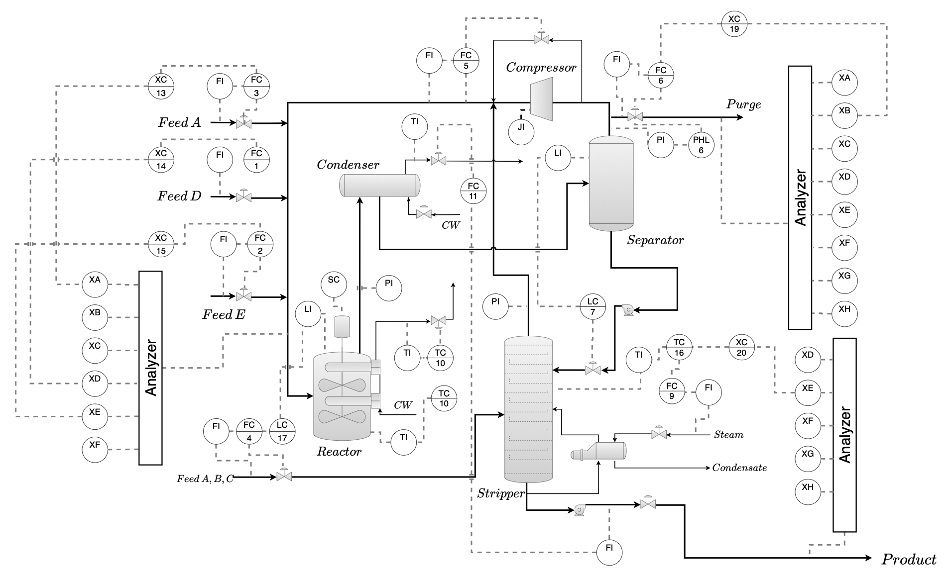
Fig. 10 The Tennessee Eastman process, the plant this session’s data comes from. Reactor, condenser, compressor, separator, and stripper, wired up with the pressure, level, temperature, and composition instruments that produce this session’s 52 columns. Figure from Lyu, Botcha, Kulkarni, Pagaria, Alves, Sunshine, and Kitchin (2026).#
Every three minutes, all 52 of those instruments report a number. Run the simulation for a few hundred batches, twenty different kinds of fault plus normal operation, and you have millions of readings before anyone has asked a single question.
Try the plant yourself
TEP Studio runs this exact simulator live in your browser: start it, watch the 52 channels trend in real time, inject one of the 20 faults, and download the resulting CSV.
Here is what we want out of all that. One row for each of the 21 conditions, showing what every sensor read on average while that condition was running. Put fault 4 next to fault 11 and you can see which sensors moved and which did not. Getting from millions of raw readings to that one small table is what this course calls a data pipeline.
Definition: data pipeline
A data pipeline is the sequence of steps that turns raw readings into an answer: load the data, clean it up, reshape it if you need to, and aggregate it into the result you actually wanted.
Lecture 3 gave you SQL: describe the result you want, and the database’s planner works out how to get it. Lecture 4 applied that same idea to a file, with DuckDB reading Parquet, still inside a database engine. So why leave the database at all? Because the work this lecture does is awkward to write as a query. You have to decide what to put in the gaps where a sensor dropped out, throw away channels that never moved, and rerun the whole thing tomorrow when the file changes. That is ordinary programming, and Python is better at it.
The catch is that you give something up when you leave. Write this as one long Python script and two things the database was handling for you are suddenly your problem:
It can be slow. A Python loop that walks the readings one at a time is hundreds of times slower than working on the whole column at once. The section below measures it.
It can be unsafe. If the script stops halfway, it leaves no record of which steps finished. You cannot tell whether running it again will pick up where it left off or double-count the work it already did.
This session rebuilds both in Python. Polars gets the speed back, along with the describe-first-run-later habit, and it needs no server. Small, restartable stages get the safety back.
Learning objectives#
By the end of this session you should be able to:
Get more familiar with pandas and, most importantly, write Polars code that operates on whole columns at once instead of row by row, including grouping and joining.
Break a data pipeline into small steps that each read one file and write one file, so a run that fails halfway through can be started again without corrupting anything.
Explain the difference between pandas running code immediately and Polars planning a computation before running it, and use that difference to choose between the two for a given task.
What carries over from SQL#
A dataframe is a table held in memory, with named columns that each have a fixed type. You have been using one since Lecture 3.
Grouping and joining you already did in Lecture 3. Vectorizing is new.
Grouping and joining. You wrote both in Lecture 3. Here they are method calls instead of clauses. readings.group_by("faultNumber") does the same job as GROUP BY faultNumber, and a join still matches two tables on a shared column, so your result can say “reactor cooling water” instead of faultNumber = 4.
Vectorizing. This one is new, because SQL never gave you the choice. You asked for a result and the database walked the rows however it wanted. Python does give you the choice, and one of the options is slow.
Definition: vectorization
Vectorization means computing on a whole column at once instead of one value at a time. readings["xmeas_7"] > threshold compares the entire column in one step, inside compiled code. A for loop compares one reading per step, in Python.
The gap is large enough to change how you write. On this session’s reactor-pressure column, 480,000 readings, the whole-column comparison takes 0.2 ms. The same test as a plain for loop takes 20 to 24 ms, and written with iterrows(), which is the idiom most people reach for first, about 3,900 ms. So the penalty runs from a hundred times to several thousand, depending on how you write the loop. All three numbers come from figures/make_figures.py, so you can rerun them on your own machine.
Polars: plan the work, then run it#
pandas runs each instruction the moment you write it, on one core. That is eager execution, the model you already know from ordinary Python. On this session’s table, 52 sensor columns and hundreds of thousands of rows, that means checking every column one at a time while the rest of your machine’s cores sit idle.
Definition: Polars
Polars is a table library for Python, like pandas, but built to use every core on your machine at once. If you ask it to, it will also plan a whole computation before running any of it.
Definition: lazy evaluation
Under lazy evaluation, writing an instruction does not run it. It adds a step to a plan. Nothing touches the data until you call .collect(), which runs the whole plan in one optimized pass.
This is Lecture 3’s query planner again, and Lecture 4’s DuckDB trick again, now with no server anywhere. pl.scan_parquet(...) hands back a description of the read, not the data. Your later steps fold back into that description before anything runs: exactly the projection pushdown and predicate pushdown DuckDB applied to Parquet in Lecture 4.
import polars as pl

pipeline = (
    pl.scan_parquet("data/tep.parquet")
    .group_by("faultNumber")
    .agg(pl.col("^xmeas_.*$").mean())   # every measured column
)
result = pipeline.collect()   # only now does anything run
The demo shows the rest live: the query plan, printed before and after optimization, and pandas-to-Polars conversion. That conversion is cheap because both libraries lay columns out the same way in memory, the Arrow format.
Making it safe to rerun#
A pipeline written as one long function has no seam: nothing to test on its own, nothing to re-run on its own. The fix is stages: load, clean, aggregate, each a small function with one input and one output, usually a Parquet file the next stage reads.
Definition: pure stage
A pure stage’s output depends only on its input, and it changes nothing else. Same input, same output, every time.
Saving each stage’s output is caching: the expensive early work runs once, and you can open any stage’s file and see exactly what it produced.
Say the clean stage is halfway through writing tep_clean.parquet when your laptop sleeps. If clean is a pure stage, the fix is one word: rerun it. Same raw file in, same output out, whether the interrupted attempt got through row one hundred or row one hundred thousand.
Definition: idempotency
A stage is idempotent when running it twice has the same effect as running it once. You do not need to know whether the last attempt finished. You just run it again.
In Lecture 3, a database’s transactions gave you this for free. Once the logic is your own Python, you rebuild it by hand: a partial failure that leaves nothing to clean up.
One trap: cache a stage’s output under a name that mentions only the stage, clean.parquet, then change a setting that stage depends on. The stale file gets reused silently, because nothing tells it to invalidate. Name the cache after the inputs and settings that actually determine its contents, not just the stage.
Where this pushes back#
Polars is stricter, and stricter costs you while you are learning it. More of your mistakes become real errors instead of quiet workarounds, and lazy evaluation moves errors away from the line that caused them, sometimes several stages away. Stay with pandas when your codebase or collaborators only speak it. Reach for Polars when a run has grown slow enough to interrupt your work, or when the pipeline is a job you run repeatedly.
A fill value is a decision you are making about the data. Whatever number you put in a gap becomes part of every result computed downstream of it. Choose it deliberately, and report how much of a column you filled alongside any summary of it.
One machine goes further than you think. Vectorized pandas, and especially Polars with DuckDB over Parquet, comfortably handle hundreds of thousands of rows on a laptop. Exhaust one good machine before adding a cluster.
A benchmark measures one workload on one machine. The pandas-versus-Polars ratio you see in the demo will not transfer to a different pipeline. The gap between a loop and a whole-column operation does transfer, because it comes from the shape of the computation, a loop against a whole-column operation, rather than from which library you picked. Measure your own pipeline before you rewrite it.
In-class demo#
We take the Tennessee Eastman readings and build the same four-stage pipeline twice, once in pandas and once in Polars, and time both. The stages are load, drop the columns that are constant or mostly missing, fill in what remains, and aggregate to the mean of each sensor per fault. The data arrives clean, so a clearly labeled cell injects the defects on purpose, dropped readings and one stuck sensor, so the cleaning stages have real work to do.
Watch the difference between eager and lazy. The pandas version builds a new table after every stage. The Polars version builds a plan and runs it in one pass at .collect(). Print that plan with .explain() and you can see the column selection folded down into the very first read: the projection pushdown from Lecture 4’s DuckDB, now with no server. The runnable notebook is l05-pipelines.ipynb.
Summary#
A data pipeline turns a raw sensor log into an answer. Lecture 3 and Lecture 4 already taught you most of how to do that well: describe the result and let a planner work out how to get it, and structure the work so a partial failure cannot corrupt anything. This session moves both ideas out of the database and into your own Python code. Vectorization and Polars get the speed back, hundreds of times over on this data. Small, pure, idempotent stages that cache to Parquet get the safety back. Whichever library you use, the two habits carry over from the last two lectures: describe the work and let the planner decide how to run it, and split the work so a failure partway through leaves nothing to untangle.
Resources#
TEP Studio. The Tennessee Eastman simulator itself, running live in your browser. Start a run, watch the 52 channels move in real time, inject a fault, and download the CSV.
Lyu, Botcha, Kulkarni, Pagaria, Alves, Sunshine, and Kitchin, Benchmarking machine learning fault detection methods on the Tennessee Eastman process dataset (2026). The plant diagram in this session comes from this paper, which benchmarks a range of machine learning fault detectors on the same dataset.
Polars user guide, Lazy API. What a
LazyFrameis, whyscan_parquetbeatsread_parquetfor a pipeline, and how.collect()triggers optimization. Start here.Polars user guide, Expressions. The expression API the whole library is built on, with the group-by and selection patterns the demo uses.
pandas user guide, Group by. The split-apply-combine model, the same idea as SQL’s
GROUP BY, in pandas.Apache Arrow overview. The in-memory columnar layout that makes pandas-to-Polars conversion cheap, and how it differs from Parquet on disk.
Tennessee Eastman process simulation data (Rieth et al. 2017). The dataset for this session. Faults 1 to 20 plus fault-free operation, 52 process variables.
Downs and Vogel, A plant-wide industrial process control problem (1993). The original paper that defines the process, its units, and its twenty disturbances. The source for what each fault means.
Assignment#
No assignment is released this session, so this week’s deliverable is the practice module below, which is where your participation credit for the session comes from.
Practice module#
Practice module for this session, about ten minutes of questions drawn from this session’s notes, slides and demo. It runs entirely in your browser, the questions are selected from your Andrew ID, and it ends by producing a PDF you upload for participation credit.