Lecture 1: The AI-engineering landscape and the modern toolchain#
Overview
Session Lecture 1, Week 1
Arc Foundations
Slides Deck for this session
Practice Practice module for this session
Demo
l01-reproducibility.ipynb, the notebook that does not reproduceAssignment 1, released this week
Why this matters#
In 2015 a group of Google engineers published a paper with an unusually blunt diagram. It drew the components of a production machine learning system as boxes sized by the code each one required. Configuration, data collection, feature extraction, serving infrastructure, and monitoring were large. The box in the middle was small, and the caption said plainly: “The box labeled ‘ML Code’ is actually tiny in proportion to the rest of the system.”
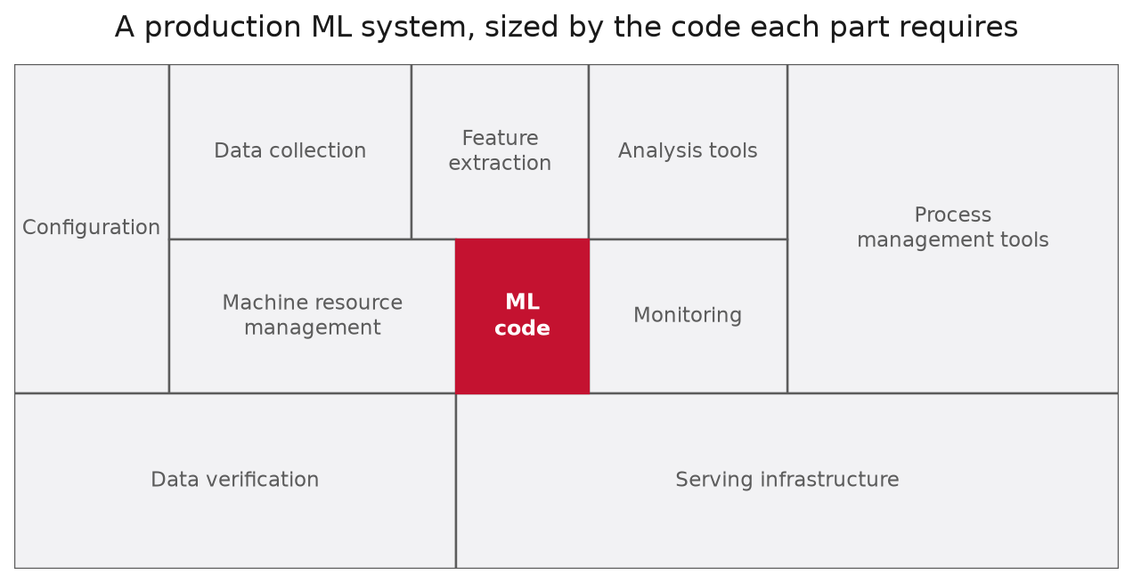
Fig. 1 Redrawn after Sculley et al. (2015). The red box is the part most courses spend the whole semester on. Everything else is this course.#
That proportion is the subject of this course. You have almost certainly trained a model in a notebook. You may not yet have had to answer the question a regulator, a safety reviewer, or a colleague joining in eighteen months will ask: can you rebuild this exact result, and can you show where the numbers came from. Those questions are not answered by a better architecture. They are answered by infrastructure.
Engineering data makes the gap wider than it is in the domains where machine learning methodology is usually taught. A sensor is not a static dataset. It drifts, it needs recalibration, it samples irregularly, it reports in physical units that must be tracked or the analysis is meaningless, and its output may end up in a safety case that has to be defensible years later. A pipeline that quietly loses provenance is unusable in that setting, because a safety case you cannot trace back to its inputs is not a safety case.
A note on the “10%” figure
You will often see this paper cited as showing that “less than 10% of the code is the model.” That number does not appear in the paper. Sculley and colleagues say only that the ML code box is “tiny in proportion to the rest of the system.” The invented precision is a small example of a habit this course will keep pushing against: check the claim against the source, and cite what the source actually says.
Learning objectives#
By the end of this session you should be able to:
Map the end-to-end lifecycle of an engineering ML system and identify the standardized toolchain used throughout the semester.
Contrast “a model in a notebook” with “a system,” naming the data contracts, drift, and monitoring concerns that separate them.
Explain why engineering data imposes provenance and traceability requirements that general-purpose ML tutorials ignore.
Justify each component of the course toolchain in terms of the failure it prevents.
The system view, and where the work actually is#
Name the stages explicitly: data acquisition, storage, pipelines, features, training, evaluation, deployment, and monitoring. Read left to right that looks like a linear process, which is the first thing to unlearn. Real systems iterate hard between features and evaluation, and the monitoring stage feeds back into acquisition when drift appears in production.
The stages also tell you where failures cluster, and it is not where students expect. Very few production incidents are caused by choosing the wrong model class. Most are caused by a schema that changed upstream without warning, a feature computed one way in training and another way in serving, or a source that silently started returning nulls. These are integration failures, and cross-validation cannot see them.
Case study: 15,841 cases that fell off the end of a spreadsheet#
In late September 2020, Public Health England was moving COVID-19 test results from a
laboratory surveillance system into the national contact-tracing system. Commercial labs
submitted results as CSV files without difficulty. PHE’s own tooling then consolidated
those results into Excel templates, and the developers had chosen the legacy .xls format,
which caps a worksheet at 65,536 rows. Because each test result occupied several rows, each
template in practice held about 1,400 cases. When a file hit the ceiling, the remaining
rows were not rejected with an error. They were simply absent.
The result was that 15,841 positive cases recorded between 25 September and 2 October 2020 were never passed to contact tracers, more than three quarters of them in the final three days. People who tested positive were told their results. Their contacts were not traced. By the following Monday, roughly half of the affected cases had still not been reached.
Nothing about this was a modeling failure. Every dashboard and epidemiological model downstream was computing correctly on the data it received. The failure was that a format decision made years earlier silently discarded records, and no process compared the count of results sent by the labs against the count arriving in the tracing system. A model cannot detect the absence of records it was never shown. That reconciliation check, the least glamorous thing in the pipeline, was the missing control.
What a practitioner should take from this
Put integrity checks at every system boundary, and make them count-based. “Did the number of records I sent equal the number that arrived” catches an entire class of silent failure that no amount of model sophistication will. Prefer formats that fail loudly over formats that truncate quietly.
Sculley and colleagues gave the general pattern a name, hidden technical debt, and their specific mechanisms are worth carrying with you. Glue code, the connective tissue that exists only to move data between systems, tends to dominate the codebase. Pipeline jungles emerge when that glue accretes without anyone redesigning it. Undeclared consumers are the most insidious: some downstream process depends on your output, you do not know it exists, and you break it.
Validating well is not evidence that a system works#
This is the hardest lesson in the course to accept, because it contradicts the way machine learning is usually taught and assessed. A model can be validated carefully, by a competent team, using a protocol stricter than most production work receives, and still be wrong for years in deployment.
Case study: Google Flu Trends#
Google Flu Trends launched in November 2008 with a genuinely attractive premise. Influenza surveillance ran on a one to two week reporting lag, and search queries were available almost immediately. If search behavior tracked influenza prevalence, you could see the epidemic sooner.
The validation was good. Screening 50 million candidate queries down to 45, fitting against regional surveillance data, the published model reported a mean correlation of 0.97 across nine regions on held-out data that had been excluded from every prior modeling step. That is a more disciplined protocol than a great deal of deployed machine learning gets even now.
In deployment it drifted badly. By the 2012 to 2013 season the system was estimating more than double the CDC’s figure for influenza-like illness. Across the 108 weeks from August 2011 to September 2013 it was too high in 100 of them. A retrospective in Science identified two mechanisms.
The first they called big data hubris, the assumption that a large dataset substitutes for rather than supplements careful measurement. In practice it showed up as overfitting: searching 50 million terms for correlations against roughly a thousand data points is nearly guaranteed to find seasonal patterns that have nothing to do with influenza. The developers had already been manually removing terms like high school basketball that correlated with flu season without being about flu, which should have been read as a warning rather than a cleaning step. The authors’ summary is the line worth remembering: the initial system was “part flu detector, part winter detector.” It failed exactly where that description predicts, missing the non-seasonal 2009 H1N1 pandemic entirely.
The second they called algorithm dynamics, meaning that the data-generating process was itself under continuous modification. Google’s search team shipped 86 changes in June and July of 2012 alone, including features that suggested related searches and surfaced possible diagnoses for symptom queries. Each was an improvement to the search product. None of the engineers involved knew that a flu model depended on the distribution of queries they were changing. This is Sculley’s undeclared consumer, appearing inside the same company.
The detail that should bother you most is the failure signature. A hundred wrong weeks out of 108, all in the same direction, is not a subtle statistical artifact. It was visible for two years. A study had already shown that simply projecting forward from three-week-old surveillance data outperformed the model. The real failure was not the model at all; it was the absence of any continuous evaluation harness comparing it against a boring baseline.
What a practitioner should take from this
Hold-out validation tells you about the distribution you sampled from, and nothing about the distribution you will meet next year. Two habits follow. Always maintain a simple-but-honest baseline in production and keep comparing against it, because a model that cannot beat a lagged average is a result you want to discover early. And check whether anything upstream of your features is under active development by a team that does not know you exist.
Why engineering data is different#
Everything above applies to machine learning generally. Three properties of engineering data sharpen it further.
Units and calibration: A model that ingests a raw sensor voltage and a model that ingests a calibrated concentration are not the same model, even with identical weights, and the difference will not appear in a validation metric. It appears when someone recalibrates the instrument.
Drift: Physical sensors degrade. The dataset we use today is a case in point: a metal-oxide gas sensor array deployed on an Italian roadside, recording hourly for about thirteen months. The documentation states explicitly that both cross-sensitivities and concept and sensor drift are present.
Rather than assert what that costs you, we can measure it. Fit a linear calibration from one sensor channel to the reference CO measurement using only the first three months, then apply it for the rest of the deployment and track the monthly error.
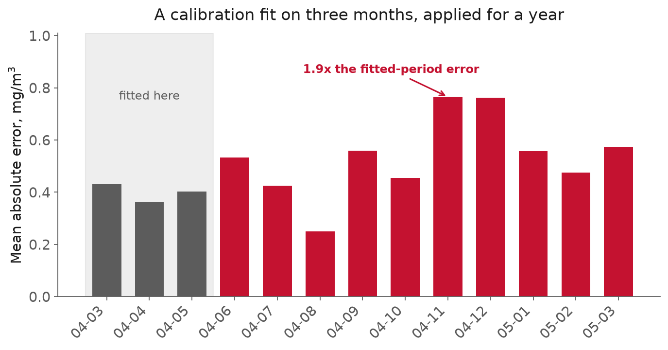
Fig. 2 Monthly mean absolute error of a calibration fitted on March to May 2004 only.#
The result is more interesting than a simple decay. The error does not creep steadily upward; it swings with the season, dipping below the fitted-period error in August and peaking at roughly 1.9 times it in November and December. The model learned spring, so it is worst exactly when conditions are least like spring. That is the same failure Google Flu Trends had, reproduced on a gas sensor: a model that is partly measuring the thing you care about and partly measuring the season.
This is also where the evaluation protocol earns its keep. Score the same data and the same model two ways, once with a random split and once by training on the earlier period and testing on the later one:
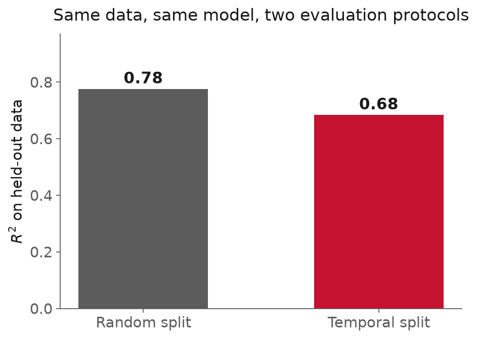
Fig. 3 The random split reports a number the deployed model will never achieve.#
The gap is small enough to pass unnoticed. A random split shuffles later readings into the training set, so the model is quietly allowed to see the future, and it reports \(R^2 = 0.78\) where the honest temporal estimate is \(0.68\). If you only ever saw the first number you would have no reason to suspect anything, which is precisely how this class of error survives review.
A note on the dataset dates
The UCI page describes this deployment as running March 2004 to February 2005. The CSV in the download actually contains hourly records through 4 April 2005, about thirteen months. The discrepancy is small and harmless here, but it is a good habit-forming example: the documentation and the artifact disagreed, and only loading the file revealed it.
Provenance: In a regulated or safety-relevant setting you may be required to reconstruct which data, which code, and which parameters produced a specific number. If the answer involves a notebook run out of order on a laptop that has since been reimaged, there is no answer. This is why reproducibility is treated here as an engineering requirement rather than as good hygiene.
Case study: a single angle-of-attack sensor#
The 737 MAX accidents are the sharpest available illustration that in engineering systems, where a number comes from is part of the safety argument. The discussion here is limited to what the accident investigations concluded.
The Maneuvering Characteristics Augmentation System (MCAS) was a control function that commanded nose-down stabilizer trim under certain flight conditions. Each aircraft carried two angle-of-attack sensors. MCAS was designed to use one of them at a time, alternating between flights, with no cross-comparison and no voting between the two. A single faulty sensor was therefore sufficient to drive the function.
On Lion Air 610 the left sensor carried a bias of roughly 21 degrees. The Indonesian investigation traced it to a replacement sensor that had been mis-calibrated during an earlier repair, with the error undetected both at the repair and by the installation test. That is a calibration provenance failure in the most literal sense: a physical measurement channel whose correctness nobody had established, feeding a control law with authority over a flight surface.
The compounding failure was in the analysis. Boeing’s hazard assessment had evaluated scenarios involving erroneous data from both air data channels and judged their combined probability beyond extremely improbable. But the actual MCAS input path was vulnerable to a single failure, so the analysis had modeled the wrong failure set. The residual risk was absorbed by an assumption that the crew would respond correctly within a few seconds, an assumption held even though the same underlying fault simultaneously produced stick shaker, airspeed disagreement, and altitude disagreement, effects the certifying simulations never reproduced because they injected the symptom rather than its cause.
The investigation’s contributing factors state the causal order plainly: incorrect assumptions about flight crew response, combined with an incomplete review of the associated flight deck effects, were what made reliance on a single sensor appear acceptable. Lion Air 610 killed 189 people in October 2018. Ethiopian Airlines 302 killed 157 in March 2019.
What a practitioner should take from this
Ask three questions of every input your system treats as ground truth. Where did this measurement come from, is it independently corroborated, and what happens downstream when it is wrong. If the answer to the third is “an operator will notice and compensate,” that is a design decision requiring evidence, not an assumption you are entitled to make.
A tour of the stack#
Definition: the stack
The stack (or toolchain) is the full set of tools and layers a system is built from, from storage at the bottom through pipelines, training, and evaluation up to serving and monitoring at the top. This course standardizes one stack, so class time goes to concepts rather than to choosing tools, and the tour below walks it one layer at a time.
The rest of this session is a quick tour, not a deep dive. Each subsection is one layer of the system diagram, so the goal today is a mental map: what each layer is for and what tends to break in it. Read it for orientation, and do not worry about mastering any single layer yet.
Storage: where engineering data actually lives#
Most engineering analysis starts life in CSV files and stops scaling almost immediately. A CSV has no schema, no types, no constraints, and no way to read a column without reading every byte in the file. The PHE incident is what the far end of that road looks like.
Three storage models cover nearly everything you will meet. Relational databases (PostgreSQL) enforce a schema and give you transactions and joins, which is what you want when data arrives continuously and correctness matters; time-series extensions handle sensor histories specifically. Columnar files (Parquet) store each column contiguously and compressed, so reading one channel out of two hundred touches only that channel, which is why they dominate analytical workloads. Embedded analytical engines (DuckDB) run SQL directly over Parquet with no server at all, which for a laptop-scale engineering dataset is frequently the entire answer. A fourth model, the vector store, indexes embeddings by similarity rather than by value.
The practitioner question is not “which database is best” but “what access pattern do I have.” Writing one row at a time while several consumers read concurrently is a relational problem. Scanning three columns across ten years is a columnar problem.
Pipelines: moving data without losing it#
A pipeline is the code that gets data from where it lands to where it is used, and it is usually the largest and least loved part of the system. Two shapes matter. Batch processing runs on a schedule over a bounded chunk of data and is what most engineering work needs. Streaming processes records as they arrive, which sensor and internet of things (IoT) contexts increasingly demand, and which buys you latency at the cost of substantially harder correctness.
The part worth internalizing now is validation. A pipeline that silently passes bad
data is worse than one that crashes, because the failure surfaces months later inside a
result nobody can explain. Declaring what you expect (column types, physical ranges, null
rates, row counts) and failing loudly when reality disagrees is the single highest-value
habit in this course. Tools like pandera and Great Expectations exist to make those
declarations executable.
Training: what actually happens#
Training is an optimization loop. You define a model with adjustable parameters, a loss function measuring how wrong it is, and then repeatedly compute the gradient of that loss with respect to every parameter and step downhill. Automatic differentiation is the machinery that makes this tractable: frameworks like PyTorch record the operations you perform and replay them backwards to get exact gradients, so you never hand-derive anything.
Deep learning matters for engineering data mainly where structure is available to exploit: convolutional models for spatial fields and images, sequence models for time series. GPUs matter because the underlying operations are large matrix multiplications, which is a problem shape GPUs are built for. But the honest framing is the one this course keeps returning to: a gradient-boosted tree on well-constructed features beats a neural network on badly constructed ones, most of the time, and the strong baseline is the thing you must beat before claiming anything.
Evaluation and experiment tracking#
Evaluation is the discipline of knowing whether the thing works, and both case studies above are evaluation failures rather than modeling failures. It divides into choosing a protocol that reflects deployment (temporal splits for time series, grouped splits when records share a source), choosing metrics that reflect the decision being made, and keeping a baseline you must beat.
Experiment tracking is the infrastructure underneath it. When you have run a hundred variants, “which configuration produced this number” becomes unanswerable from memory, and the provenance requirement from earlier becomes unmeetable. MLflow records parameters, metrics, and artifacts per run, so one run equals one reproducible fact.
Packaging and deployment: containers#
Your model runs on your laptop. That is not a deliverable. Deployment is the work of making it run somewhere else, repeatedly, for someone who is not you.
Containers are the standard answer. A container image bundles your code with its
dependencies, system libraries, and interpreter into a single artifact that runs
identically anywhere the runtime exists, which is a much stronger guarantee than a
requirements.txt. Docker is the usual tool for building and running them. The mental
model worth carrying: a virtual machine virtualizes hardware and boots a whole operating
system, whereas a container shares the host kernel and isolates only the process, which is
why containers start in milliseconds and VMs in tens of seconds.
Around the container you need a way to be called. FastAPI and similar frameworks expose your model as an HTTP endpoint with typed request and response schemas, which is also a data contract with your callers. Then the questions become operational rather than statistical: latency budget, throughput, cost per prediction, and what happens under load.
Monitoring and operations#
Deployment is where most courses stop and where the actual lifetime of a system begins. Models degrade because the world moves, exactly as the calibration figure above shows. Monitoring means watching input distributions for drift, watching predictions for distribution shift, and watching the gap against ground truth once labels eventually arrive.
Machine learning operations (MLOps) is the practice of automating that loop: continuous integration that tests data and models rather than only code, reproducible retraining, staged rollout so a bad model does not reach everyone at once, and the ability to roll back. Flu Trends is what this looks like when it is absent.
Language models and agents#
A large language model (LLM) is a next-token predictor trained on a very large corpus, and almost everything surprising about it follows from scale plus that simple objective. For systems purposes the details that matter are practical: text is split into tokens, the model sees a bounded context window, you pay per token in both money and latency, and outputs are sampled rather than deterministic.
Three integration patterns cover most engineering use. Prompting puts instructions and data in the context. Retrieval-augmented generation searches your own corpus, usually via embeddings in a vector store, and puts the retrieved passages in the context, which is how you ground answers in documents the model never trained on. Fine-tuning adjusts the weights, and is the right answer far less often than people expect.
An agent extends this with tool use. The model is given descriptions of functions it may call, it emits a structured request to call one, your code executes it and returns the result, and the loop repeats until the task is done. That is the whole idea; the frameworks are conveniences around it. For engineering work the interesting version is agents over your own tools, querying a database, running a simulation, or driving an instrument.
Security and responsibility#
Adding a language model to a system adds attack surface that most engineers have not met before. Prompt injection is the central one: if untrusted text reaches the context window, that text can carry instructions, and the model has no reliable way to distinguish data from commands. Any agent that both reads untrusted input and holds a capability to act is exposed to this by construction, which is why capability scoping matters more than clever prompting.
Beyond that sit the concerns that predate LLMs and still dominate in engineering settings: who is allowed to see this data, what happens if the model is wrong in the direction that hurts, whether the training data licenses what you are doing with it, and whether the system’s failure modes are documented well enough for someone to sign a safety case. MCAS is a reminder that these questions have answers with consequences.
The standardized toolchain#
We fix one toolchain across all of the above so class time goes to concepts rather than tool selection. Each choice exists to prevent a specific failure, and it is worth naming the failure rather than the feature.
Layer |
Tool |
The failure it prevents |
|---|---|---|
Environments |
Python + |
rebuilds that are merely probable |
Storage |
PostgreSQL, DuckDB, Parquet |
CSV sprawl, silent truncation |
Dataframes |
pandas, Polars |
out-of-memory, unreadable transforms |
Validation |
pandera |
bad data passing silently |
Tracking |
MLflow |
results nobody can attribute |
Deep learning |
PyTorch |
hand-derived gradients |
Retrieval |
a vector store |
answers ungrounded in your corpus |
Serving |
FastAPI, Docker |
“works on my machine” |
The LLM and agent material is deliberately framework-agnostic and provider-agnostic. That part of the ecosystem turns over faster than a semester, so the course teaches the interfaces and the evaluation discipline rather than a specific vendor’s abstractions.
Common pitfall
The most frequent reproducibility break is not an exotic dependency conflict. It is an absolute file path, an unpinned random seed, or hidden notebook state from running cells out of order. Get in the habit of “Restart and Run All” before you trust any notebook result, including your own.
In-class demo#
We walk a single notebook that ingests the UCI Air Quality data, plots a reference CO measurement against the corresponding sensor response, and fits a naive train/test split. It works, and it looks convincing.
Then we run the same notebook on a fresh checkout, where it breaks three times. Your job is to diagnose each break before I do: a missing package version, an unpinned seed producing different numbers, and an absolute path that existed only on my machine. None of the three is exotic, and none of them announces itself as a reproducibility failure while you are making it.
The notebook is l01-reproducibility.ipynb. Run it before class if
you like, but do not fix anything yet.
Summary#
A model is a small component inside a system whose bulk is data infrastructure, evaluation, and operations, and that is where both the engineering effort and the failures concentrate. Three cases make the shape of it concrete. Public Health England lost 15,841 records to a file format and a missing count check, with no model involved. Google Flu Trends validated at a correlation of 0.97 and was then wrong in the same direction for a hundred weeks because nobody was watching it against a baseline. MCAS treated one uncorroborated sensor as ground truth, and the safety analysis had modeled a different failure than the one the design was exposed to. Engineering data sharpens all of this by adding units, calibration, drift, and traceability. The toolchain we standardize on is not arbitrary; each piece answers a specific way that undisciplined work falls apart.
Resources#
Hidden Technical Debt in Machine Learning Systems. Sculley et al., NeurIPS 2015. The source of the framing above, and of glue code, pipeline jungles, and undeclared consumers. Nine pages, and worth reading in full.
The Parable of Google Flu: Traps in Big Data Analysis. Lazer, Kennedy, King and Vespignani, Science 2014. Three pages, and the source of every GFT figure quoted above.
Detecting influenza epidemics using search engine query data. Ginsberg et al., Nature 2009. Read this one before the Lazer critique, so you see how reasonable it looked at the time.
PHE statement on delayed reporting of COVID-19 cases. the official statement, for the 15,841 figure and the dates.
Excel: Why using Microsoft’s tool caused Covid-19 results to be lost. BBC, for the technical mechanism. The clearest published account of how the truncation actually happened.
The Design, Development & Certification of the Boeing 737 MAX. US House Committee on Transportation and Infrastructure, September 2020. Long; the single-sensor discussion is around p. 106.
UCI Air Quality Data Set. dataset description and citation. Read the note on cross-sensitivities and drift before Thursday.
uv documentation, Getting started. Install it before class, because we build live.
The Turing Way, Reproducible Research. The broader case, if the motivation section left you unconvinced.
For the tour of the stack#
None of these are required reading. They are the place to start on any layer that sounded unfamiliar, and each is the source I would send a colleague to first.
DuckDB documentation. Start here if the storage section was new. Reading Parquet with SQL and no server is a ten-minute experiment worth doing.
Apache Parquet file format. Why columnar layout changes what is cheap to read.
pandera. Executable data contracts. The quickest way to see the point of the validation argument.
PyTorch, A Gentle Introduction to torch.autograd. What automatic differentiation is actually doing.
MLflow Tracking Quickstart. One run equals one reproducible fact, in practice.
Docker, What is a container?. The container mental model, briefly.
FastAPI. Typed HTTP endpoints, which double as a data contract with your callers.
OWASP Top 10 for LLM Applications. The standard catalog of LLM-specific security risks, prompt injection first among them.
NIST AI Risk Management Framework. The vocabulary regulators and safety reviewers are increasingly using.
Practice module#
Practice module for this session, about ten minutes of questions drawn from the numbers and the pitfalls above. It runs entirely in your browser, the questions are selected from your Andrew ID, and it ends by producing a PDF you upload for participation credit.