Lecture 4: Columnar storage, Parquet, and DuckDB#
Overview
Session Lecture 4, Week 2
Arc Data Systems
Slides Deck for this session
Practice Practice module for this session
Demo
l04-storage.ipynb, the Intel Lab data stored columnar and queried three waysAssignment 2, released this session; it draws on Lecture 3’s material and this one’s
Why this matters#
At the end of Lecture 3 the Intel Berkeley Lab readings sat in a relational database, indexed on (sensor_id, ts) so that a narrow query, one sensor over one hour, came back in a few hundredths of a millisecond. That is the query a live dashboard makes, and the row-oriented database from Lecture 3 is very good at it.
It is not good at the other kind of question. An analyst does not ask about one sensor for one hour; they ask for the average temperature of every mote over the whole month, the daily energy across the floor for a year, or how one channel is distributed across the entire history. Those questions do not narrow to a few rows. They read one or two columns across all of the rows, and an index has nothing to prune, so the database reads the whole table.
The reason that is slow comes down to how the data sits on disk. A relational database keeps each row’s columns together, one row after another, because that makes writing a reading or fetching a whole row cheap. But it means that to average one column you still have to pull every other column of every row off the disk to reach it. Our readings table has six columns; to compute an average temperature the database reads humidity, light, voltage, the identifiers, and the timestamps too, on all 2.3 million rows, and then discards almost all of it.
The fix does not change what the data means, only how the bytes are arranged: store each column’s values together instead of each row’s. Then the average-temperature query reads only the temperature values, in one contiguous run, already compressed. That single change is the subject of this session. We keep the exact Lecture 3 dataset and move it into columnar Parquet files, read by an embedded engine called DuckDB, and we measure what it buys. On these 2.3 million readings the same “average temperature per mote” query runs about 80 times faster from Parquet through DuckDB than from a row store, and the Parquet file is about 5.5 times smaller on disk than the same data as CSV. The rest of the session is why that works, and when it is the right trade.
Learning objectives#
By the end of this session you should be able to:
Explain the row-store versus column-store trade-off and why a columnar layout is faster to scan, and read and write Parquet.
Query Parquet with DuckDB, and choose between a transactional (OLTP) and an analytical (OLAP) tool.
Name the other kinds of store (document, key-value, time-series) and say when each one fits.
Row stores and column stores#
Every database has to decide, at the lowest level, how to place a table’s values on disk, and there are two natural answers. The logical table looks identical either way; what changes is which values end up physically next to each other, and that decides what is cheap.
Definition: row store
A row store keeps each row’s columns together on disk: all of row one, then all of row two, and so on. Reading or writing a whole row is cheap, which is why it suits transactional work. PostgreSQL from Lecture 3 is a row store.
Definition: column store
A column store keeps each column’s values together: every row’s timestamp, then every row’s mote id, then every temperature. Scanning one column is cheap, because its values are contiguous and the columns you do not ask for are never read.
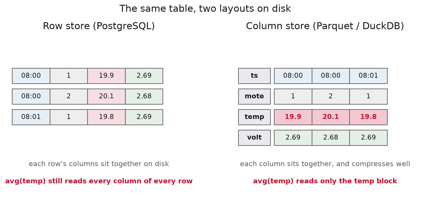
Fig. 8 The same table on disk, two ways. A row store keeps each row’s columns together, so a scan of one column still pulls every other column off the disk. A column store keeps each column together, so the same scan reads only the block it needs, and each column, holding one kind of value, compresses well.#
These two layouts suit two different jobs, and the industry has names for them. Getting the names straight is worth it, because they are the vocabulary for the rest of the session and for the assignment.
Definition: OLTP (online transaction processing)
OLTP is the work of many small operations that touch whole rows: insert a reading, update a record, fetch this one row by its key. A row store is the right layout, because a whole row lives in one place. This is what Lecture 3’s PostgreSQL is built for.
Definition: OLAP (online analytical processing)
OLAP is the work of scanning a few columns across enormous numbers of rows to compute an aggregate or a trend. A column store is the right layout, because the columns it needs live together and the columns it ignores are never read.
The most useful question this session gives you is not “which database is better,” but “is this workload OLTP or OLAP,” because the honest answer for a real platform is usually that it runs both.
Why a column layout is fast#
A column layout buys its speed in three ways that stack on top of each other.
Definition: column projection
Column projection: a query that names two columns reads only those two, so the cost scales with the columns you ask for rather than the width of the whole table.
The second reason is compression. A column holds one kind of value, and neighboring values are often similar: a temperature near the last temperature, a mote id repeated thousands of times. That compresses far better than the mixed bytes of a row, and smaller data is less to read from disk, which is itself a speedup. It is most of why the Parquet file ends up 5.5 times smaller than the CSV.
Definition: predicate pushdown
Predicate pushdown: a columnar reader keeps a small summary of each block, the minimum and maximum value in it, and uses that to skip whole blocks that cannot match a WHERE clause, without reading them at all.
A note on the measurement
The 80-times figure is the same avg(temperature) GROUP BY mote over the whole table, as it grows from 0.2 to 2.3 million rows, run against a row store and against Parquet read by DuckDB. Two honest caveats. The row store here is SQLite, chosen because it needs no running server, standing in for the row-oriented layout rather than benchmarking PostgreSQL specifically. And part of the speedup is DuckDB’s execution engine, not the layout alone. The shape is the durable lesson: the row store’s cost climbs with the table (about 46, 138, 310, 608 ms) while the columnar cost barely moves (about 1.5 to 7.6 ms), because one reads everything and the other reads two columns of six.
Parquet: a columnar file format#
Columnar is an idea about layout. Parquet is the file that stores data that way, and it has become the standard on-disk form for it, so you will produce and read it constantly.
Definition: Parquet
Parquet is an open columnar file format. It stores a table column by column, compresses each column on its own, and carries its own schema inside the file, so any tool that speaks Parquet can read it with no server and no separate description of the data.
Parquet does not store each column as one giant run, which would make writing and partial reads awkward. It divides the rows into row groups, and within each row group it stores each column together, encoded and compressed on its own. A footer at the end of the file records the schema and, for each column in each row group, small statistics including the minimum and maximum value.
Definition: row group
A row group is a horizontal slice of a Parquet file, perhaps a few hundred thousand rows. Within it, each column is stored and compressed separately, and the footer’s per-column min/max statistics are what let a reader skip a row group that cannot match a filter.
Two practical things follow. Because each column is compressed on its own and holds one kind of value, Parquet routinely stores engineering data in a fraction of the space of the CSV it came from. And because it is just a file, or a folder of files, it needs no server: you write it, copy it, and any tool that reads Parquet can read it. You will most often write it from pandas with df.to_parquet(...), or from PyArrow (the Python library for Apache Arrow) directly, and read it back the same way.
The one structural choice Parquet asks of you is partitioning: instead of one enormous file, write a folder tree whose folder names encode a column’s value, for example readings/date=2004-03-01/part.parquet, so a query filtered to one date opens only that folder. Partition on a column you filter by often, date or sensor for our readings, and do not let the partitions get too small, because thousands of tiny files carry their own overhead.
Common pitfall
Parquet is a file format, not a database, and it is easy to expect database behavior it does not have. A Parquet file has no indexes you build, no transactions, and no in-place edit: to change a row you rewrite the file that holds it, and to add data you write new files rather than appending to old ones. That immutability suits analytics, where data arrives in batches and is read far more than written. The moment your work is really point updates, that is a sign the data belongs in the row store from Lecture 3, not in Parquet.
DuckDB: SQL analytics inside your process#
If Parquet is where analytical data rests, DuckDB is the engine that reads it.
Definition: DuckDB
DuckDB is an embedded analytical (OLAP) database: it runs inside your own process, with no server to start, no connection to manage, and no data to load in first. You import duckdb and you are querying. The useful shorthand is that DuckDB is to analytics what SQLite is to transactions.
What makes it worth a lecture is that it collapses the distance between your files and your queries. DuckDB reads Parquet directly, with no import step:
SELECT mote_id, avg(temperature)
FROM 'readings/*.parquet'
GROUP BY mote_id;
There is no CREATE TABLE and no load phase. DuckDB reads the Parquet where it sits, and because it is a columnar engine reading a columnar format, it applies exactly the two savings from the last sections: it reads only the columns the query names (projection), and it uses the per-row-group statistics to skip groups that cannot match a WHERE clause (predicate pushdown). Writing is just as direct, with COPY (SELECT ...) TO 'out.parquet' (FORMAT parquet).
That leaves the question of where pandas fits, since you already use it for data that lives in memory. pandas is the right tool when the data fits comfortably in memory and you want to compute in Python. DuckDB is the better tool when the data is larger than memory, when the work is naturally written as SQL, or when you want to query files without first pulling everything into a dataframe. They also interoperate: DuckDB can query a pandas dataframe directly and hand the result back as one, so the choice is rarely all-or-nothing. The contrast to carry is the measured one:
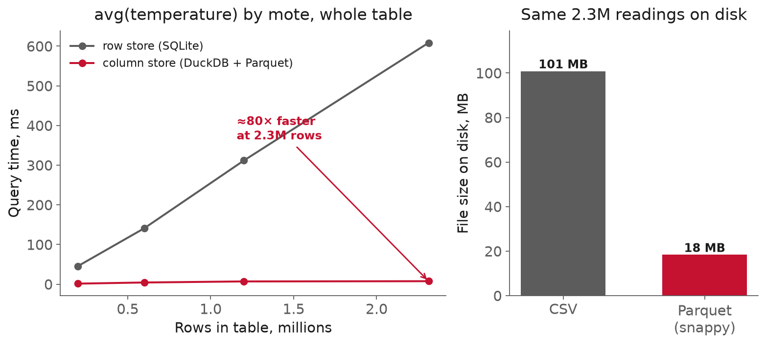
Fig. 9 The same analytical query, avg(temperature) per mote over the whole table, as it grows toward 2.3 million rows (left), and the same readings stored as CSV versus Parquet (right). The row store’s cost grows with the table because it reads every column of every row; the columnar reader stays nearly flat because it reads two columns of six.#
The other stores, in one line each#
The relational database and the columnar file cover most engineering data between them. A few other kinds of store exist for access patterns that leave the table behind. You should recognize them, not build them here. Each one gives up a relational guarantee you learned to value in Lecture 3, usually the fixed schema or the joins, in exchange for a better fit to one access pattern.
Document store (for example, MongoDB): stores flexible, JSON-like records whose fields can vary from one record to the next. Right for irregular experiment metadata where every run records a different set of parameters; wrong for uniform sensor readings, where the schema is the point.
Key-value store (for example, Redis): a fast dictionary, a value stored and fetched by its key, often entirely in memory. Right for a cache or a small hot lookup; not for rich queries or joins.
Time-series database (for example, InfluxDB): a database specialized for very high-rate timestamped writes, with time bucketing and retention built in.
The rule for all of them is the same: reach for one because your access pattern demands it, not because designing a schema felt like work.
Where columns and DuckDB stop helping#
This session has argued for columnar storage and for DuckDB, and it is a strong argument, but each advantage was an advantage for one access pattern. Reaching for the same tool outside that pattern gets you the worst of both.
Columnar is the wrong home for writes and updates#
The layout that makes analytical scans fast makes changes slow. A Parquet file is effectively immutable: you add data by writing new files, and you change a value by rewriting the file that holds it, because there is no in-place update. For data that arrives in batches and is read far more than written, that is fine. For data that is constantly corrected one record at a time, it is a poor fit, and that record belongs in the row store from Lecture 3.
Small data needs none of this#
The 80-times speedup shows up at millions of rows. At a few hundred thousand it shrinks, and for data that fits comfortably in memory a pandas groupby is simpler, fast enough, and one fewer moving part. The columnar machinery pays off at scale; below that scale, reaching for it is over-engineering, the same lesson Lecture 2 made about scaffolding a throwaway script.
OLTP and OLAP compose#
The most common mistake after this lecture is to conclude that DuckDB and Parquet replace the relational database. They do not. A real platform typically runs both: PostgreSQL takes the live writes with its schema and transactions intact, and the history is periodically written out as Parquet that DuckDB scans for analytics. The choice is not loyalty to a row store or a column store; it is putting each part of the workload where its access pattern is cheap.
What a practitioner should take from this
Store data in the shape that matches how it will be read. Continuous writes, point lookups, and strong consistency mean a row store and OLTP, which is the relational database of Lecture 3. Wide scans and aggregates over history mean a column store and OLAP, which is Parquet plus an engine like DuckDB, and the payoff there is large (about 80 times here). Most serious systems run both and move data across the seam on purpose. Reach past all of these to a document, key-value, or time-series store only when your access pattern leaves the relational model behind, and never just to avoid designing a schema.
In-class demo#
We pick up the Intel Lab readings where Lecture 3 left them and change only where they live. Starting from the data, we write it out as partitioned Parquet, then ask the same analytical question, the average temperature per mote over the whole table, three ways: as a pandas groupby, as SQL against a row store, and as SQL against the Parquet through DuckDB, comparing both the lines of code and the wall-clock time. Then we use DuckDB’s zero-import reach: querying the Parquet files directly with no load step, and watching a filtered query prune partitions.
The moment to watch is the analytical scan. The row store’s time climbs with the table while the columnar read stays nearly flat, because one reads every column and the other reads two. The runnable notebook is l04-storage.ipynb.
Summary#
Storage layout should match access pattern. The relational row store from Lecture 3 is built for transactions and point lookups and is the right home for live, continuously written data; it is the wrong tool for scanning one channel across the whole history, because a row store reads every column of every row. A column store fixes exactly that, and Parquet is its standard file form: columnar, compressed per column, partitioned for pruning, and self-contained. DuckDB is the embedded engine that reads Parquet with no import step, applying projection and predicate pushdown so a query touches only what it needs. On the Intel Lab readings the difference is about 80 times in query time and 5.5 times in file size, measured rather than assumed. Around these two stores sit a few others, document for irregular metadata, key-value for caches, time-series for high-rate ingestion, each a deliberate trade of a relational guarantee for a fit to one access pattern. The skill this session builds is matching the store to how the data will be read.
Resources#
DuckDB, Reading and writing Parquet. Querying Parquet directly with
FROM 'file.parquet'and writing it withCOPY ... TO. The place to start.DuckDB, Parquet tips. How projection and row-group skipping (via per-column min/max statistics) actually cut the work.
DuckDB, Why DuckDB. The in-process, OLAP design goals in the project’s own words.
Apache Parquet, File format and overview. Row groups, column chunks, and the footer metadata, from the source.
Kleppmann, Designing Data-Intensive Applications, Ch. 3. “Column-Oriented Storage” is the clearest explanation of why row and column stores make opposite choices (1st edition; chapter numbering differs in the 2nd).
MongoDB, Document databases. What a document store is and when a flexible, per-record schema fits.
InfluxDB, Get started. A purpose-built time-series platform, for the high-ingest end of the landscape.
Redis. The in-memory key-value store, for caches and hot lookups.
Intel Lab Data. The dataset carried over from Lecture 3, now stored columnar. Served over plain HTTP.
Assignment#
Assignment 2, “Sensor data into PostgreSQL + DuckDB,” is released this session and is due roughly one week later. Its first half is Lecture 3’s material, loading the sensor data into PostgreSQL and querying it with SQL; its second half is this session’s, moving the same dataset into Parquet and DuckDB and comparing the two. With both halves now covered, you can do the whole assignment. This is a pointer, not the rubric.
Practice module#
Practice module for this session, about ten minutes of questions drawn from this session’s notes, slides and demo. It runs entirely in your browser, the questions are selected from your Andrew ID, and it ends by producing a PDF you upload for participation credit.