
L13 worked example: a physics-informed network in JAX#
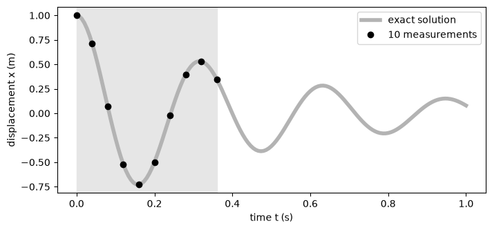
A damped spring-mass, measured during its first 0.36 s. A plain network and a physics-informed neural network (PINN) learn from the same ten points. Where is the mass after the data run out?
\(m = 1\) kg, \(\mu = 4\) N·s/m, \(k = 400\) N/m.
1. The data#
exact(t) is the closed-form solution: it makes the data and scores the models.
Run this first on Colab#
Colab starts from its own preinstalled environment rather than this course’s uv
environment, so run the cell below before anything else. It installs what this
notebook needs and Colab does not already have. Outside Colab it does nothing, so
you can run it or skip it.
# Run this first on Colab. Anywhere else this cell does nothing.
#
# Only genuinely missing packages are installed, so Colab's own versions of
# everything it already ships are left alone.
import importlib.util
import subprocess
import sys

REQUIREMENTS = {
    "jax": "jax",
    "matplotlib": "matplotlib",
    "numpy": "numpy",
    "optax": "optax",
}


def _missing(module):
    try:
        return importlib.util.find_spec(module) is None
    except ModuleNotFoundError:  # the parent package is absent
        return True


if "google.colab" in sys.modules:
    need = sorted({pip for mod, pip in REQUIREMENTS.items() if _missing(mod)})
    if need:
        print("installing:", " ".join(need))
        subprocess.run([sys.executable, "-m", "pip", "install", "-q", *need], check=True)
    print("Colab setup done." if need else "Colab: nothing to install.")
import jax
import jax.numpy as jnp
import matplotlib.pyplot as plt
import numpy as np
import optax

jax.config.update("jax_enable_x64", True)

m, mu, k = 1.0, 4.0, 400.0


def exact(t):
    d = mu / (2 * m)
    w = np.sqrt(k / m - d**2)
    return np.exp(-d * t) * (np.cos(w * t) + d / w * np.sin(w * t))


t_data = np.linspace(0, 0.36, 10)       # 10 measurements, first 0.36 s
x_data = exact(t_data)
t_phys = np.linspace(0, 1, 40)          # 40 collocation points, the whole second
t_plot = np.linspace(0, 1, 151)
x_true = exact(t_plot)

fig, ax = plt.subplots(figsize=(8, 3.5))
ax.plot(
    t_plot,
    x_true,
    color="0.7",
    lw=4,
    label="exact solution",
)
ax.plot(t_data, x_data, "ko", label="10 measurements")
ax.axvspan(0, 0.36, color="0.9")
ax.set_xlabel("time t (s)")
ax.set_ylabel("displacement x (m)")
ax.legend()
plt.show()
2. The network#
Three hidden layers of 32 tanh units. x_nn takes one time, the form jax.grad needs.
def init(key, sizes):
    params = []
    for n_in, n_out in zip(sizes[:-1], sizes[1:]):
        key, sub = jax.random.split(key)
        W = jax.random.normal(sub, (n_in, n_out)) * np.sqrt(1 / n_in)
        params.append((W, jnp.zeros(n_out)))
    return params

def net(params, t):
    h = t[:, None]
    for W, b in params[:-1]:
        h = jnp.tanh(h @ W + b)
    W, b = params[-1]
    return (h @ W + b)[:, 0]

def x_nn(params, t):
    return net(params, jnp.array([t]))[0]

params0 = init(jax.random.PRNGKey(0), [1, 32, 32, 32, 1])
print("weights and biases:", sum(W.size + b.size for W, b in params0))
weights and biases: 2209
3. The two losses#
The data loss uses the ten measurements. The physics loss uses the residual at the 40 collocation points:
dx = jax.grad(x_nn, argnums=1)      # dx/dt
ddx = jax.grad(dx, argnums=1)       # d2x/dt2

def residual(params, ts):
    x = jax.vmap(lambda t: x_nn(params, t))(ts)
    v = jax.vmap(lambda t: dx(params, t))(ts)
    a = jax.vmap(lambda t: ddx(params, t))(ts)
    return m * a + mu * v + k * x

def data_loss(params):
    return jnp.mean((net(params, jnp.array(t_data)) - x_data) ** 2)

def physics_loss(params):
    return jnp.mean(residual(params, jnp.array(t_phys)) ** 2)

lam = 1e-4

def pinn_loss(params):
    return data_loss(params) + lam * physics_loss(params)
residual0 = residual(params0, jnp.array([0.5]))[0]
print("residual of the untrained network at t = 0.5 s:", float(residual0))
residual of the untrained network at t = 0.5 s: -94.28226097449125
4. Training#
Adam, 30,000 steps, the same start for both networks: only the loss differs. About 10 s.
def train(loss, steps=30_000):
    opt = optax.adam(1e-3)
    params = params0
    state = opt.init(params)

    @jax.jit
    def step(params, state):
        grads = jax.grad(loss)(params)
        updates, state = opt.update(grads, state, params)
        return optax.apply_updates(params, updates), state

    for _ in range(steps):
        params, state = step(params, state)
    return params

p_nn = train(data_loss)
p_pinn = train(pinn_loss)
5. After the data run out#
x_nn_plot = np.asarray(net(p_nn, jnp.array(t_plot)))
x_pinn_plot = np.asarray(net(p_pinn, jnp.array(t_plot)))
after = t_plot > t_data[-1]


def rmse(a, mask):
    return np.sqrt(np.mean((a[mask] - x_true[mask]) ** 2))


print(f"{'':30s}{'network':>10s}{'PINN':>10s}")
print(f"{'RMSE inside the data (m)':30s}{rmse(x_nn_plot, ~after):10.4f}{rmse(x_pinn_plot, ~after):10.4f}")
print(f"{'RMSE after the data (m)':30s}{rmse(x_nn_plot, after):10.4f}{rmse(x_pinn_plot, after):10.4f}")
for name, p in [("network", p_nn), ("PINN", p_pinn)]:
    grid = float(jnp.sqrt(jnp.mean(residual(p, jnp.array(t_plot)) ** 2)))
    colloc = float(jnp.sqrt(physics_loss(p)))
    print(f"{name}: residual RMS {grid:.1f} N over the second, {colloc:.2f} N at the collocation points")

fig, ax = plt.subplots(figsize=(9, 3.8))
ax.axvspan(0, 0.36, color="0.9")
ax.plot(
    t_plot,
    x_true,
    color="0.7",
    lw=5,
    label="exact",
)
ax.plot(
    t_plot,
    x_nn_plot,
    color="C1",
    lw=2,
    label="plain network",
)
ax.plot(
    t_plot,
    x_pinn_plot,
    "C0--",
    lw=2,
    label="PINN",
)
ax.plot(t_data, x_data, "ko", label="data")
ax.set_xlabel("time t (s)")
ax.set_ylabel("displacement x (m)")
ax.legend(ncol=4)
plt.show()
                                 network      PINN
RMSE inside the data (m)          0.0067    0.0008
RMSE after the data (m)           0.5418    0.0010
network: residual RMS 163.0 N over the second, 165.39 N at the collocation points
PINN: residual RMS 5.3 N over the second, 0.70 N at the collocation points
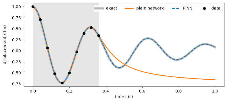
The plain network drifts to a flat line once the data stop; the PINN follows the oscillation. Its residual is small, but not zero: the physics is a penalty.