Lecture 16: Generative AI, learning a distribution and sampling from it

At a glance

• Session Lecture 16, Week 8

• Arc Machine learning and deep learning

• Slides Deck for this session

• Practice Practice module for this session

• Demo l16-generative-optimization.ipynb, a Gaussian mixture and a flow-matching model that find every root of the Peng-Robinson cubic and the optimum of a batch reactor by conditional sampling

• Tools scikit-learn’s GaussianMixture, PyTorch for flow matching

• Assignment None released with this session

Why this matters

Here is a question that looks too easy to get wrong. You have 240 measurements of a quantity \(y\) that depends on a setting \(x\) through \(y = |x|\), with a little noise, and for some reason no measurements were taken for \(-0.5 < x < 0.5\). Which setting gives \(y = 0.75\)? The approach from Lecture 9 is to fit a model of \(x\) as a function of \(y\) and ask it. A least-squares line through these data answers \(x \approx 0.00\). The true answers are \(x = -0.75\) and \(x = +0.75\). The fitted value is their average, and it is not an answer at all: no measurement anywhere near it gives \(y = 0.75\).

A more flexible model does not rescue this. A Gaussian process or a neural network trained by minimizing squared error on data with two branches also predicts the mean of the branches, because the mean is what minimizes squared error. Regression learns one number per input, \(E[x \mid y]\), and an inverse question with two answers does not have one number.

Engineering is full of such questions. The Peng-Robinson equation of state for propane at 300 K and 10 bar is a cubic in the compressibility factor \(Z\) with three real roots: a liquid root at \(Z = 0.0348\), an unstable middle root at \(0.1280\), and a vapor root at \(0.8147\). Newton’s method returns whichever root its starting guess happens to lead to. In the right panel of the figure below, starts spread uniformly over \([0, 1]\) reach the liquid root 20% of the time, the unstable root 37% and the vapor root 43%. Nothing in the answer tells you the other two exist, and the basins are not even contiguous: starts between about 0.45 and 0.57 jump all the way down to the liquid root.

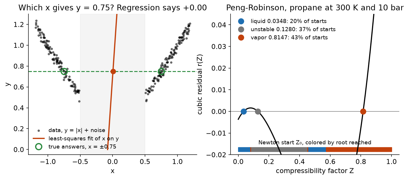
Fig. 126 Two inverse questions with more than one answer. Left: a least-squares fit of \(x\) on \(y\) returns the average of the two answers. Right: Newton’s method on the Peng-Robinson cubic finds one root, chosen by the starting guess. Both panels are generated by figures/make_figures.py.

This session is about models that answer such questions properly. A generative model learns the whole distribution of the data, inputs and outputs together, instead of one function from inputs to an output. Once you have the distribution you can fix any variables you know and sample the rest, which returns every answer consistent with what you fixed. The same idea is underneath every product called “generative AI”: an image generator, a molecule generator and a chatbot all learn a distribution from data and sample from it, usually conditioned on something you supplied. Seeing the idea in two dimensions, where every sample can be checked, is the clearest way to understand what those large systems are doing and where they fail.

Learning objectives

By the end of this session you should be able to:

• Distinguish a generative model from the regression and classification models of L8–L14, and explain why a regression model gives a wrong answer to an inverse question with more than one solution.

• Fit a Gaussian mixture model to the joint distribution of inputs and outputs, choose the number of components, and condition it to sample the inputs that give a target output.

• Explain how flow matching turns samples of a simple distribution into samples of the data, train one with a mean-squared-error loss, and sample it by integrating an ODE.

• Pose root finding, optimization and parameter estimation as conditional sampling, and check the samples against the physical model.

• Place generative models in the machine-learning landscape, and explain why they are as dependent on data, and as limited by it, as any regression model.

• Describe how generative models are used for images, molecules, proteins, materials and weather, and the failure modes those uses share.

What a generative model learns

Treat every row of a data set as a draw from an unknown probability distribution. For the \(|x|\) data a row is the vector \((x, y)\), and the distribution \(p(x, y)\) is a density over the plane that is high along the two branches of the V and zero elsewhere. A generative model is a model of that distribution, learned from the rows.

Definition: generative model

A generative model learns the probability distribution of the data well enough to draw new samples from it, and sometimes to evaluate the probability density at a point.

Those two abilities, sampling and evaluating the density, are separate. Some models do both; some, including the flow-matching models later in this session, only sample. Sampling is the one that matters for the inverse questions above.

The rows do not have to be measurements of a function. An image is a grid of pixel values, and flattening the grid gives a long vector: a 512 × 512 color image is a vector of 786,432 numbers. A collection of photographs is then a cloud of points in a space of that dimension, with strong correlations between neighboring coordinates, and generating a new photograph means drawing a new point from that cloud and reshaping it into a grid. Alves and Kitchin make this observation the starting point of their paper on generative optimization (ChemRxiv, 2026), the anchor reading for this session. A row of inputs, outputs and derivatives from an engineering model is the same kind of vector, only much shorter. Whatever works for images works in principle for \((Z, r(Z))\), and the short vector has the advantage that every sample can be checked.

Joint, marginal and conditional

Three distributions come out of one data set. The joint distribution \(p(x, y)\) describes the inputs and outputs together. A marginal, such as \(p(y)\), ignores some variables: it is the histogram of \(y\) alone. A conditional, such as \(p(x \mid y = 0.75)\), fixes some variables and describes the rest: it is the slice of the joint along the line \(y = 0.75\), renormalized. For the \(|x|\) data that slice has two peaks, at \(\pm 0.75\), and sampling it returns both answers in proportion to how much data supports each.

Conditioning is the operation that turns a generative model into a solver. Fix the outputs and sample the inputs, and you have solved an inverse problem. Fix the inputs and sample the outputs, and you have a forward prediction with its uncertainty. Fix some of each and you have a question that regression cannot even express, such as “given this feed temperature and this product purity, what reflux ratio and steam rate are consistent with the plant’s history?”

Discriminative and generative models

The models of Lectures 8 to 14 are discriminative: they learn \(p(y \mid x)\), or often only its mean \(E[y \mid x]\), and they answer in one direction. A generative model of the joint answers in any direction, at the price of modeling more. The table sets the two side by side.

	Discriminative (regression, classification)	Generative
What is learned	\(E[y \mid x]\) or \(p(y \mid x)\)	\(p(x, y)\), or a way to sample it
Which questions	inputs to outputs	any variables given any others
What comes back	a number, or one distribution over \(y\)	samples, every mode included
What it must model	how \(y\) depends on \(x\)	that, and how \(x\) is distributed

Three ways to make a distribution learnable

Writing down a distribution over many variables is hard, and there are three common ways to make it tractable. They organize the rest of this session.

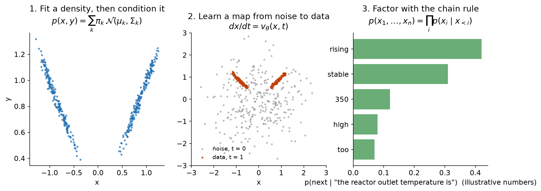
Fig. 127 Three ways to make \(p(x)\) learnable. The bar heights in the right panel are illustrative, not the output of a model.

The first is to choose a flexible family of densities and fit its parameters, then condition it with algebra. A mixture of Gaussians is the standard example, and it is the first approach developed below. The second is to give up on writing the density and instead learn a transformation that carries an easy distribution, usually a standard normal, onto the data. Normalizing flows, diffusion models and flow matching all work this way; this is the second approach below. The third is to factor the joint with the chain rule of probability,

\[p(x_1, x_2, \ldots, x_n) = p(x_1)\,p(x_2 \mid x_1)\,p(x_3 \mid x_1, x_2) \cdots = \prod_i p(x_i \mid x_{<i}),\]

which is exact, and to learn each conditional “what comes next, given everything so far.” Sampling then draws \(x_1\), then \(x_2\) given \(x_1\), and so on. This is called an autoregressive model. It is the family that language models belong to, where each \(x_i\) is a word or a piece of a word; this session names it and leaves it there.

Learning the joint distribution: Gaussian mixture models

The first approach writes the joint density down explicitly. One Gaussian is too simple for a V-shaped cloud, but a weighted sum of several Gaussians can follow any smooth shape if it has enough of them.

Definition: Gaussian mixture model

A Gaussian mixture model writes a density as a weighted sum of \(K\) Gaussians, \(p(\mathbf{z}) = \sum_{k=1}^{K} \pi_k\, \mathcal{N}(\mathbf{z}; \boldsymbol{\mu}_k, \boldsymbol{\Sigma}_k)\), with weights \(\pi_k\) that sum to one.

Start with one Gaussian over \((x, y)\). Its mean vector says where the cloud is, and its covariance matrix says how the cloud is stretched and tilted. The off-diagonal covariance \(\Sigma_{xy}\) is the linear relationship between \(x\) and \(y\), so a single Gaussian is linear regression viewed as a joint distribution. A mixture of \(K\) Gaussians covers a curved relationship with \(K\) locally linear pieces. For the \(|x|\) data two components suffice, one tilted ellipse along each branch.

Fitting by expectation maximization

The parameters are the weights, means and covariances of every component. They are fitted by maximizing the likelihood of the data, and the standard algorithm is expectation maximization (EM), introduced in its general form by Dempster, Laird and Rubin (1977). EM alternates two steps. The E-step computes, for every data point, a responsibility for each component: the probability that the point came from that component under the current parameters. The M-step recomputes each component’s weight, mean and covariance as averages over the data, weighted by those responsibilities. Each pass cannot decrease the likelihood. If you have seen k-means clustering, EM is k-means with soft assignments and with clusters that have shapes, which is why Gaussian mixtures are also a clustering method.

EM converges to a local maximum, and which one depends on where it starts. scikit-learn’s GaussianMixture runs it from several starts (n_init) and keeps the best. The interactive figure below runs EM in your browser; press Play to watch the ellipses find the branches, and try \(K = 1\) to see one Gaussian give up on the V entirely.

Choosing the number of components

More components always raise the likelihood on the training data, so the likelihood alone cannot choose \(K\). The Bayesian information criterion (BIC) adds a penalty proportional to the number of parameters, and the \(K\) with the lowest BIC is a reasonable default. For the \(|x|\) data, BIC falls from 543 at \(K = 1\) to \(-697\) at \(K = 2\) and rises again to \(-673\) at \(K = 4\): two components are best, matching the two branches. Held-out log-likelihood, computed on data the mixture did not see, is the other honest check, and it is the same idea as the held-out test sets of Lectures 8 to 10.

Conditioning a mixture

A Gaussian has a property that makes it unusually convenient: fix some of its coordinates, and the distribution of the rest is again Gaussian, with a mean and covariance given in closed form. Partition the variables into the ones you fix (\(k\), for known) and the ones you want (\(u\)), and partition the mean and covariance to match. Given the known values \(\mathbf{v}\),

\[\boldsymbol{\mu}_{u \mid k} = \boldsymbol{\mu}_u + \boldsymbol{\Sigma}_{uk}\boldsymbol{\Sigma}_{kk}^{-1}(\mathbf{v} - \boldsymbol{\mu}_k), \qquad \boldsymbol{\Sigma}_{u \mid k} = \boldsymbol{\Sigma}_{uu} - \boldsymbol{\Sigma}_{uk}\boldsymbol{\Sigma}_{kk}^{-1}\boldsymbol{\Sigma}_{ku}.\]

The second expression is called the Schur complement. The first says the conditional mean moves from the unconditional mean along the regression line of \(u\) on \(k\); the second says the conditional spread is the original spread minus what the known values explain.

For a mixture, condition each component \(j\) this way and then reweight the components by how well each one explains the known values, \(\pi_j\,\mathcal{N}(\mathbf{v}; \boldsymbol{\mu}_{k,j}, \boldsymbol{\Sigma}_{kk,j})\), renormalized. Here \(\boldsymbol{\mu}_{k,j}\) and \(\boldsymbol{\Sigma}_{kk,j}\) are component \(j\)’s mean and covariance restricted to the known variables. The result is again a Gaussian mixture, so sampling it is exact and immediate. At \(y = 0.75\) the two branch components each explain the value equally well, each conditional is a narrow Gaussian centered near its branch’s answer, and the samples split between \(x \approx -0.75\) and \(x \approx +0.75\). Move the \(y^*\) slider in the figure above to watch the lower panel; the orange line is the regression’s single answer.

The surprise here is that the split between inputs and outputs is chosen after training. The same fitted mixture answers \(p(x \mid y)\), \(p(y \mid x)\), and any mixed question, because conditioning is a function call with the known columns as an argument. Nothing about which variables are inputs was decided when the model was fitted. The notebook’s condition function, about twenty lines of NumPy, is the whole method. The gmr library (Fabisch, 2021) packages the same computation as Gaussian mixture regression.

Root finding, optimization and parameter estimation

Alves and Kitchin turn this into a uniform recipe for problems that are normally solved by specialized algorithms. In each case you generate or collect rows containing the variables you will search over and a quantity you want to fix, fit the joint, and condition.

Root finding. Sample \(Z\) uniformly on \([0.01, 0.99]\), evaluate the Peng-Robinson residual \(r(Z)\) at each sample, fit a mixture to the 2,000 rows \((Z, r)\), and condition on \(r = 0\). All three roots come out of one set of samples. The paper’s Table 1 reports 0.035 ± 0.001, 0.128 ± 0.010 and 0.814 ± 0.002, against true roots of 0.0348, 0.1280 and 0.8147. The course’s own fit, twelve components on standardized \((Z, r)\), puts the clusters at 0.0440, 0.1273 and 0.8143. The vapor and unstable roots are within 1%, and the liquid root is 26% high. The liquid root sits in a narrow region of \(Z\) where the cubic changes quickly, so the result there is sensitive to fitting choices such as \(K\), the scaling of the columns and the random seed. One fix that works here is to fit the same mixture to \((\log Z, r)\), which spreads the small values of \(Z\) out. That gives 0.0346 for the liquid root, at the cost of a slightly worse unstable root, 0.1257 (1.8% low). Choosing the representation is part of the modeling, as it was for the features of Lecture 7.

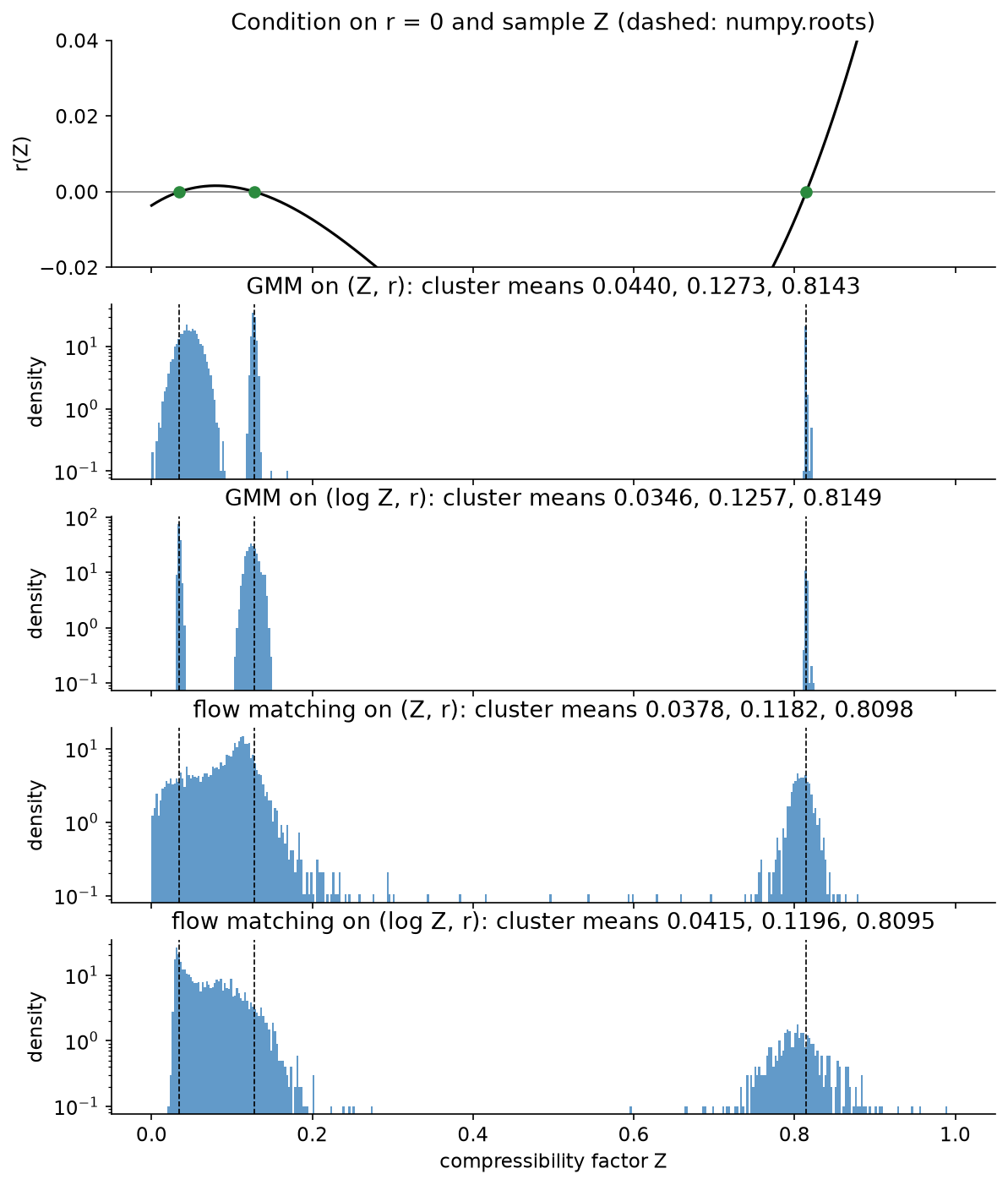
Fig. 128 Condition on \(r = 0\) and sample \(Z\). Panel titles give the mean of the samples within 0.03 of each true root. The GMM in \(\log Z\) recovers all three; flow matching blurs the two close roots. Generated by figures/make_figures.py.

The samples are starting points, and the honest last step is to polish the center of each cluster with a few Newton iterations against the real cubic. In the notebook that turns 0.0440, 0.1273 and 0.8143 into 0.0348, 0.1280 and 0.8147, identical to numpy.roots. The generative model’s contribution is to find every basin at once; the solver’s contribution is precision.

Unconstrained optimization. At an interior optimum the derivative is zero, so condition on it. For consecutive reactions \(A \to B \to C\) in a batch reactor with \(k_1 = 0.5\) and \(k_2 = 0.2\ \mathrm{min}^{-1}\), the intermediate \(C_B(\tau)\) peaks at \(\tau^* = \ln(k_1/k_2)/(k_1 - k_2) = 3.05\) min. Sample \(\tau\), compute \(C_B\) and \(dC_B/d\tau\) (by automatic differentiation, as in Lecture 11), fit the joint distribution, and condition on \(dC_B/d\tau = 0\). The paper fits \(p(\tau, C_B, dC_B/d\tau)\); the notebook drops \(C_B\) and fits \(p(\tau, dC_B/d\tau)\), which is enough for this question. The paper’s GMM gives a mean of 2.89 min and its flow-matching model 3.04 min. In the notebook, the GMM’s samples have a median of 3.13 min, with the middle 90% between 2.93 and 3.33 min. Conditioning on a zero derivative finds every stationary point. A function with a maximum and a minimum would return both, and a second condition or the second-derivative test tells them apart.

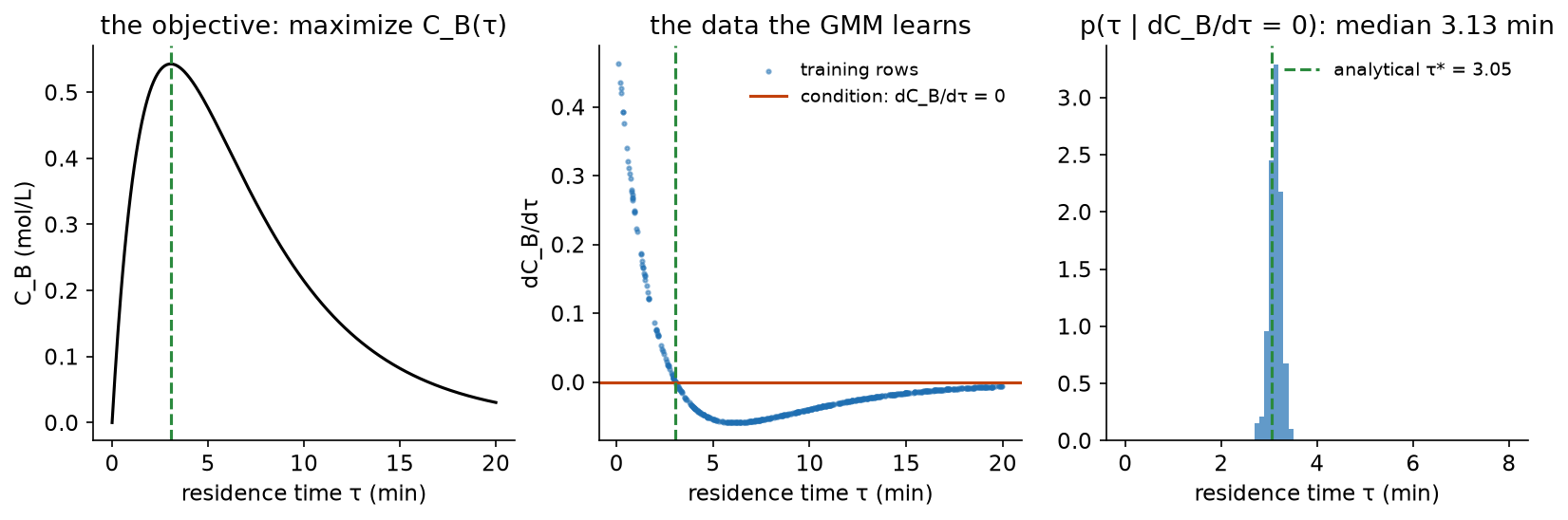
Fig. 129 Optimization by conditioning. Left: the objective. Middle: the rows the mixture learns, and the condition \(dC_B/d\tau = 0\). Right: residence times sampled from the conditioned mixture, against the analytical optimum. Generated by figures/make_figures.py, with the notebook’s data and seeds.

Constrained optimization. With constraints the objective’s gradient is not zero at the optimum, but the gradient of the Lagrangian is, so the paper adds the Lagrange multipliers as columns and conditions on all the partial derivatives of the Lagrangian being zero. One example is a gasoline blend of reformate, isomerate and alkylate that must meet an octane specification. There the GMM’s samples average \(x = (0.284, 0.607, 0.109)\), the same as the scipy SLSQP solution, with standard deviations below 0.01 in each fraction. Inequalities are handled with a log-barrier term instead.

Parameter estimation. Simulate a plug-flow reactor for many pairs of rate constants \((k_1, k_2)\), record the exit flows \((F_A, F_B)\), fit the joint of all four, and condition on the flows you observed. The answer is a distribution over rate constants, the set of parameters consistent with the observation, rather than one fitted pair. Its width is the kind of uncertainty Lecture 14 asked you to interpret with care: it mixes noise in the data with the surrogate’s own error.

Where Gaussian mixtures stop

A full covariance matrix in \(D\) dimensions has \(D(D+1)/2\) entries, and every component has one, so a mixture’s parameter count grows with \(D^2\) and EM’s cost with \(D^3\). Gaussian mixtures are a good tool for tens of variables. They are hopeless for an image, where \(D\) is in the hundreds of thousands, and they struggle with relationships that are sharp or strongly curved, which need many components. That limit is what the second approach removes.

Transforming a simple distribution: flows, diffusion and flow matching

The second approach never writes the data’s density down. Instead it learns a function that transforms samples of a simple distribution, usually a standard normal, into samples of the data. You already know one generator that works this way.

Inverse transform sampling

To draw from any one-dimensional distribution, draw \(u\) uniformly on \([0, 1]\) and return \(x = F^{-1}(u)\), where \(F\) is the target’s cumulative distribution function. This is inverse transform sampling, and it is a generative model with a known transformation. Where the target density is high, \(F\) is steep, so a given range of \(u\) maps onto a narrow range of \(x\), and samples pile up there.

That piling up is the change of variables rule. If \(x = g(z)\) with \(g\) invertible, the densities are related by \(p_X(x) = p_Z(z)\,\left|\det \partial z / \partial x\right|\): a map that compresses volume raises the density, and one that stretches volume lowers it. Any learned transformation has to keep track of that factor if it is going to report a density. In one dimension the transformation is the inverse CDF, which you can tabulate. The difficulty is learning one in many dimensions.

Normalizing flows

A normalizing flow builds the transformation from a stack of invertible layers, each designed so its Jacobian determinant is cheap to compute, and fits it by maximum likelihood using the change-of-variables formula (Rezende and Mohamed, 2015; the review by Papamakarios et al., 2021, is the standard reference). Flows give an exact density and exact sampling. The price is the architecture: every layer must be invertible with a tractable determinant, which rules out most of the network designs from Lecture 12. Invertible networks have been used directly for engineering inverse problems (Ardizzone et al., 2019).

Continuous flows

Instead of stacking layers, let the transformation be the solution of an ordinary differential equation. Start a point at \(x(0)\) drawn from the normal distribution and move it with a velocity field,

\[\frac{dx}{dt} = v_\theta(x, t), \qquad 0 \le t \le 1,\]

and call \(x(1)\) the sample. This is the neural ODE of Lecture 13, used to move a whole distribution of starting points instead of one trajectory (Chen et al., 2018, who called these continuous normalizing flows). Any smooth velocity field gives an invertible map, so the architecture restriction disappears. Training by maximum likelihood, however, means solving the ODE inside every training step, which is slow.

Diffusion models

Diffusion models take a different route to the same kind of map. A fixed forward process adds a little Gaussian noise to the data at each of many steps until nothing but noise is left. A network is trained to undo one small step at a time. Generating a sample means starting from noise and applying the learned reverse steps (Sohl-Dickstein et al., 2015; Ho, Jain and Abbeel, 2020). Song et al. (2021) showed that the process can be written as a stochastic differential equation, and that it has a deterministic twin, the probability flow ODE, which is a continuous flow of the kind above. Diffusion is the method behind most image generators of the last several years, and it is the approach the weather, protein and materials models in the survey below use.

Flow matching

Flow matching keeps the continuous flow and replaces its expensive training with regression (Lipman et al., 2023, who describe it as a simulation-free way to train continuous normalizing flows; Liu, Gong and Liu, 2023, who call the same idea rectified flow). It is the simplest of these methods to understand and to implement, so it gets the full treatment here.

Definition: flow matching

Flow matching trains a velocity field \(v_\theta(x, t)\) by regression onto the velocities of straight lines from noise samples to data samples, then generates data by integrating \(dx/dt = v_\theta\) from noise at \(t = 0\) to \(t = 1\).

One training example is built in four steps. Draw a data sample \(x_1\), a noise sample \(x_0 \sim \mathcal{N}(0, I)\), and a time \(t\) uniformly on \([0, 1]\). Form the point on the straight line between them,

\[x_t = (1 - t)\,x_0 + t\,x_1 .\]

The velocity of that line is \(x_1 - x_0\). Train the network to predict it, with the mean-squared-error loss \(\mathcal{L}(\theta) = \mathbb{E}\,\lVert v_\theta(x_t, t) - (x_1 - x_0) \rVert^2\). That is the whole training procedure: a regression, with the same optimizer and loss as Lecture 9 and Lecture 11, and no ODE is solved during training. To generate, draw \(x_0\) from the normal distribution and integrate \(dx/dt = v_\theta\) from \(t = 0\) to 1. The paper uses 100 Euler steps, \(x \leftarrow x + v_\theta(x, t)\,\Delta t\). Its version of the path adds a small noise floor \(\sigma\) so the target stays finite near \(t = 1\), which changes nothing essential.

To make the model conditional, give the network the condition as an extra input, \(v_\theta(x_t, c, t)\), and train on pairs \((x_1, c)\) from the data. For the \(|x|\) problem, \(x_1\) is \(x\) and \(c\) is \(y\). At sampling time you choose \(c\), and the flow carries noise to \(p(x \mid c)\). In the figure below, set \(y^*\) and press Play: sixty noise samples flow to the two branches. The gray arrows are the velocity field.

The field in that figure is not a trained network. For a finite data set \(\{x_{1,i}\}\), the velocity field that minimizes the flow-matching loss has a closed form. At each point \((x, t)\) it is the average of the straight-line velocities of the training points whose lines could pass through \(x\) at time \(t\), weighted by how likely that is:

\[v^*(x, t) = \sum_i w_i(x, t)\,\frac{x_{1,i} - (1 - \sigma)\,x}{1 - (1 - \sigma)\,t}, \qquad w_i \propto \mathcal{N}\!\left(x;\ t\,x_{1,i},\ (1 - (1 - \sigma)\,t)^2\right).\]

The figure computes this field exactly in your browser, with the paper’s noise floor (\(\sigma = 0.02\)). It conditions on \(y^*\) by multiplying each weight by a Gaussian kernel of width 0.04 in \(y\), so strictly it is the minimizer for those kernel-weighted data. It shows what a network is trying to learn. The field is exact for the data, so its samples land on training points. A network cannot represent the field that exactly, and its smoothness is what lets it produce samples between the training points. That is also the first sign of a failure mode discussed under the limitations below: a model that fits its training data too well reproduces it.

Why the paths curve

Every training example is a straight line, yet the trajectories in the figure curve, and samples split between the branches only partway through. The reason is that the network sees many lines through each point and learns their average velocity. Near \(t = 0\), a point at \(x = 0.1\) lies on lines heading to both branches, so its average velocity is small; only later, when the lines through a point all head the same way, does the field commit. The figure below makes this concrete in two dimensions. On the left, noise samples move along straight lines to randomly paired data points, which is what training examples look like, and the lines cross. On the right, the same noise samples follow the averaged field. An ODE assigns one velocity to each point at each time, so no two particles are ever at the same place at the same time, although a path may pass where another path was earlier. At every \(t\) the two clouds have the same distribution, and the readout compares their means and spreads. Rectified flow (Liu, Gong and Liu, 2023) and minibatch optimal transport (Tong et al., 2024) are ways of choosing the pairs so the paths are straighter and fewer integration steps are needed.

The same problems, by flow matching

On the \(|x|\) data, a conditional flow-matching model sends samples conditioned on \(y = 0.75\) to both branches, with means near \(-0.74\) and \(+0.76\). The model is a three-layer network of 64 units, trained for 4,000 minibatches in about ten seconds on a CPU. On the Peng-Robinson roots it finds the vapor root, but it blurs the liquid and unstable roots into one broad band between 0 and 0.15, and changing to \(\log Z\) does not separate them. Between those two roots \(|r|\) never exceeds 0.0016, which is 3.6% of the standard deviation of \(r\) across the training data, so the condition \(r = 0\) barely distinguishes them. The Gaussian mixture conditions in closed form and resolves them; the network has to learn the conditioning, and it learns it smoothly. The paper’s Figure 4 shows flow matching resolving all three roots, with its own architecture (sigmoid activations) and longer training (500 epochs). The comparison here is one data point about sensitivity to those choices.

Where generative models fit in machine learning

Every model in this session is a statistical model fitted to data by optimization, the same kind of object as the models of earlier lectures. Placing generative models among those methods is the fastest way to predict what they can and cannot do.

Supervised, unsupervised and generative

Machine learning is usually divided by what the data contains. Supervised learning fits a map from inputs to labeled outputs, which is what Lectures 8 to 12 did. Unsupervised learning finds structure in unlabeled data: clusters, low-dimensional representations, densities. Generative modeling began on the unsupervised side, as density estimation, and the Gaussian mixture was a clustering method long before anyone used it as a solver. A conditional generative model, however, is trained on pairs \((x, c)\) exactly as a supervised model is; it just learns the whole conditional distribution instead of its mean. Models trained on very large unlabeled corpora blur the line further, because the “label” for each piece of the data is another piece of the same data, which is called self-supervised learning.

The more useful distinction for an engineer is between kinds of question. Use a discriminative model when every input has one answer and you only need that answer. Use a generative model when an answer can have several values, when you need to ask in more than one direction, or when you need samples, for instance to propagate uncertainty or to propose candidates.

Generative models also sit next to Bayesian inference. A Bayesian treatment of an inverse problem combines a prior on the parameters with a likelihood from a forward model and samples the posterior, usually by Markov chain Monte Carlo, which requires evaluating the forward model many times. A generative model learned from simulated or measured pairs reaches the same kind of answer, a distribution over parameters given an observation, without a likelihood at inference time. This is the idea behind simulation-based inference (Cranmer, Brehmer and Louppe, 2020). The cost moves to training, and the result is only as good as the data and the fit.

Still data-driven

A generative model is a surrogate model of the data, and everything Lecture 9 and Lecture 14 said about surrogates applies to it without exception.

It needs data, and it needs more than a regression for the same job. A regression models how \(y\) depends on \(x\); a generative model of the joint also models how \(x\) is distributed, which is extra work that has to be paid for in samples. Density estimation gets harder quickly as the dimension grows, which is why the image and molecule models in the survey below are trained on millions of examples.

It is only valid where the data are. Conditioning on a value outside the training data does not raise an error. The model returns samples anyway, built from whatever its building blocks do far from data. The notebook asks both models about \(y = 0.3\), inside the gap, where the true answers are \(\pm 0.30\), and both answer without hesitation. The Gaussian mixture says \(-0.31\) and \(+0.31\), close to right only because its straight ellipses extend the straight branches; it would be wrong for a curved function. The flow-matching model says \(-0.41\) and \(+0.33\). This is the extrapolation failure of earlier lectures, and it is harder to see here, because in many dimensions it is not obvious which conditions are inside the data.

It inherits the data’s flaws. Bias in what was measured, gaps in the operating range and mislabeled rows all end up in the samples. A model of a plant’s historian data learns the plant as it was operated, including the operating policy, so it cannot tell you about regions the operators never visited. That can be useful, because the historian already encodes the constraints the plant runs under, which is the argument the paper makes for its evaporator example. It is also a limit, because the optimum might be somewhere the plant has never been.

It answers questions about the surrogate. Every sample is a solution of the learned distribution, which may or may not be a solution of the system. When an exact model exists, it should check the samples, as the Newton polishing above did. When only data exist, the samples are hypotheses to test, and the generative model is the cheapest way to propose them.

And it is still a model with hyperparameters: the number of components, the network size, the training length, the number of integration steps, and the representation of the variables, as the \(\log Z\) result showed. Each needs the held-out evaluation and seed-to-seed comparison the earlier lectures required of any model.

Pros and cons against the alternatives

The table compares three ways of answering an inverse or optimization question: a conventional solver applied to a model, a discriminative surrogate, and a generative model.

	Solver on a model (Newton, SLSQP, IPOPT)	Discriminative surrogate	Generative model
Needs a model of the system	yes	no, needs data	no, needs data
Answers in which direction	the one it was posed in	inputs to outputs	any direction
Several solutions	one per starting point	averages them	all, as samples
Accuracy	to solver tolerance	surrogate error	surrogate error, plus sampling
Cost of a new value of the condition	a new solve	one evaluation	one batch of samples
Certificate of optimality	KKT conditions checked	none	none
Scales to high dimension	yes, with structure	yes	flows and diffusion yes, GMMs no

Alves and Kitchin are explicit that generative optimization does not replace mathematical programming. Its strengths are finding every solution at once, working from data when no model exists, and answering a new condition without solving again. Its weaknesses are the weaknesses of the surrogate underneath it.

Choosing between the two approaches

Within generative models, the two approaches of this session trade off in a predictable way.

	Gaussian mixture	Conditional flow matching
What is learned	a density: weights, means, covariances	a velocity field (a neural network)
Training	EM, seconds	gradient descent, seconds here, hours or more at scale
Sampling	an exact draw	an ODE solve, about 100 network calls per sample
Conditioning	any variables, chosen after training	only the variables fed to the network in training
Density at a point	exact	not directly available
Dimension	tens of variables	up to millions

The conditioning row is the one most often missed. A Gaussian mixture can be asked \(p(x \mid y)\) today and \(p(y \mid x)\) tomorrow. A conditional flow-matching model trained to generate \(x\) given \(c\) can only answer that question; asking a different one means training a different model.

Generative models in science and engineering

The same two ideas, learn a distribution and sample it conditionally, run through the large systems that made generative AI a household phrase and through a growing body of scientific work. For each domain below, ask the same two questions: what is generated, conditioned on what, and how were the samples checked?

Images

Two model families came before diffusion. Generative adversarial networks (Goodfellow et al., 2014) train a generator against a discriminator that tries to tell generated samples from real ones. Variational autoencoders (Kingma and Welling, 2013) learn an encoder into a low-dimensional latent space and a decoder back out, and generate by decoding random latent points. Both are transformation models in the sense of this session: they map a simple distribution onto the data.

The current generation of image models is built on diffusion and flow matching. Rombach et al. (2022) ran diffusion in the latent space of an autoencoder rather than on pixels, which made high-resolution generation affordable. The Stable Diffusion models are latent text-to-image diffusion models of this kind, conditioned on a text prompt. Esser et al. (2024) scaled rectified flow, the straight-path flow matching above, to text-to-image models, and Stability AI’s Stable Diffusion 3 uses that formulation. The two-dimensional flow in this session’s figures and a text-to-image model share a training objective and differ in scale, architecture and conditioning signal.

Molecules

Molecules are discrete graphs, which makes them awkward to generate. Gómez-Bombarelli et al. (2018) trained a variational autoencoder on SMILES strings, so that molecules became points in a continuous latent space that could be searched by gradient-based optimization for desired properties. The paper is candid about the central problem: without care the latent space has “dead areas” that decode to invalid SMILES strings, which is why every molecule a generator proposes has to be checked for validity before anyone believes it. Later work generates 3-D structures directly, with diffusion models that respect rotations and translations (Hoogeboom et al., 2022), and uses diffusion to generate the pose of a drug molecule docked in a protein (DiffDock, Corso et al., 2023).

Proteins

RFdiffusion (Watson et al., 2023) generates protein backbones by diffusion, conditioned on design requirements such as a binding target or a symmetry. Its check was the laboratory. The authors characterized the structures and functions of hundreds of designed proteins experimentally. The cryo-electron microscopy structure of a designed binder in complex with influenza haemagglutinin was “nearly identical to the design model.” AlphaFold 3 (Abramson et al., 2024) predicts the joint structure of proteins, nucleic acids and small molecules with what its authors call a “substantially updated diffusion-based architecture”: structure prediction itself has become conditional generation, with the sequence as the condition.

Materials

The Crystal Diffusion Variational Autoencoder (Xie et al., 2022) generates periodic crystal structures. MatterGen (Zeni et al., 2025) is a diffusion model for inorganic materials that can be fine-tuned to generate structures with a target property. The authors generated 8,192 candidates for each of four target bulk moduli, selected four for synthesis after expert inspection, and succeeded with one: TaCr₂O₆, in a compositionally disordered version of the ordered structure the model predicted. The target was 200 GPa, and DFT on the ordered structure gave 222 GPa. The measurement was indirect: nanoindentation measured a Young’s modulus, and the bulk modulus was estimated from it with a DFT-computed Poisson ratio. The paper reports the estimate as “up to 169 GPa after four measurements (158 ± 11 GPa).” The abstract’s “within 20% of our target” holds at 169 GPa, the upper end of that range. At the central value, 158 GPa, the estimate is 21% below the target. The synthesis is a real result, and the headline figure depends on which end of the reported range you read. Park, Li and Walsh (2024) ask the broader question directly in the title of their perspective, “Has generative artificial intelligence solved inverse materials design?”

Weather

GenCast (Price et al., 2025) is a conditional diffusion model that generates the next global weather state, conditioned on the current and previous states, and rolls forward to build a forecast. Because each sample is a different plausible future, an ensemble of samples is a probabilistic forecast, which is generation used as uncertainty quantification in the sense of Lecture 14. It produces a 15-day forecast at 0.25° resolution in about 8 minutes on one Cloud TPU v5 device. It had greater skill than the European Centre’s operational ensemble, ENS, on 97.2% of the 1,320 combinations of variable, lead time and level evaluated. Its check is the standard one in forecasting: it was trained on reanalysis from 1979 to 2018 and scored against what the weather actually did in 2019.

Process engineering and optimization

The anchor paper applies the methods of this session to root finding, optimization, parameter estimation and the mapping of a desired output region back to the design inputs that produce it. Its capstone is an evaporator flowsheet with twelve process equations. The training data were optimal and suboptimal solutions over a grid of constraint settings, with noise added to mimic plant measurements. The models were conditioned on the active constraints and on all twelve equation residuals being zero. The best GMM sample reached an optimality gap of 1.61% against the scipy SLSQP solution, and the best flow-matching sample 5.83%. Both best samples were near-feasible, with a largest constraint violation just under the paper’s threshold of 0.1. Kitchin (2025) works through a single inverse problem with generative models in more detail, and the review by Anstine and Isayev (2023) surveys generative models across the chemical sciences.

What a practitioner should take from this

• In every successful example above, the generator proposes and something else verifies: a laboratory, a held-out season of weather, DFT, or the physical model. Plan the verification before you train the generator.

• Read the measurement behind a headline number, as with MatterGen’s 169 GPa against a central value of 158 GPa.

• Validity checks are part of the method. A generated molecule, crystal or operating point is not an answer until it has passed them.

Limitations and trade-offs

The limitations follow from what a generative model is: a fitted surrogate of a data distribution, sampled at random.

The samples answer questions about the surrogate. A sample is consistent with the learned distribution, which can differ from the system. The course fit’s liquid root at 0.0440 instead of 0.0348 is the small version of this; a generated molecule that cannot be synthesized is the large one. Check samples against the real model wherever one exists.

Conditioning outside the data returns confident output. There is no warning when a condition is outside the training data. In two dimensions you can see the gap; in two hundred you usually cannot, and in high dimensions it is not even obvious how to define “inside.”

Sharp structure is missed. Features that the data do not resolve, such as two roots separated by a residual that never exceeds 0.0016, are blurred or lost, in fitting and in sampling. More data where the structure is, or a better representation such as \(\log Z\), helps more than a bigger model.

Conditioning can be fixed at training time. A conditional flow-matching model answers only the question it was trained for. Gaussian mixtures are flexible here and limited in dimension.

Validity is not built in. Generated molecules can violate valence, generated crystals can be unstable, and generated operating points can violate constraints the data did not make explicit. The paper’s constrained examples succeed because the constraints were added as conditions.

Models memorize. A generative model fitted too closely to its training set reproduces training examples, as the exact flow field in this session’s figure does by construction. Carlini et al. (2023) generated 175 million images from Stable Diffusion, 500 for each of the 350,000 most-duplicated training captions. They found 94 that matched training images closely enough to count as extracted under their definition, and 13 more near-copies on manual inspection. For engineering data that means a model trained on proprietary or personal records can leak them.

Training on generated data degrades a model. Shumailov et al. (2024) showed that models trained recursively on the output of earlier models lose the tails of the original distribution, and that this “model collapse” occurs in language models, variational autoencoders and Gaussian mixture models alike. Generated samples are not new data, and a pipeline that feeds them back in as training data is making the model narrower.

Evaluation has no single number. A regression has a test error. A generative model’s samples can be individually plausible and collectively wrong, missing a mode or overweighting one. For engineering problems the best evaluation is usually the physical model: compute the residual, the constraint violation or the property for every sample, as the root-finding and evaporator examples did.

In-class demo

The notebook l16-generative-optimization.ipynb follows the notes. It shows the regression failure on the \(|x|\) data, then a Gaussian mixture chosen by BIC and conditioned with a twenty-line function, then a conditional flow-matching model in PyTorch with its trajectories. Both models are asked about the gap. The Peng-Robinson roots are found by three models and polished with Newton’s method, and the batch-reactor optimum is found by conditioning on a zero derivative. It runs on a CPU in a few minutes and is adapted from the anchor paper’s repository, which has many more examples and a SKILL.md for working through them with an LLM assistant.

Summary

A generative model learns the distribution of the data instead of one function of it, and conditioning that distribution answers questions in any direction, returning every answer consistent with what you fixed. Gaussian mixtures write the joint density down, fit it by expectation maximization and condition it exactly with the Schur complement; they are fast, flexible in what they condition on, and limited to tens of variables. Flow matching learns a velocity field that carries noise to data, trains by plain regression on straight-line velocities, and samples by integrating an ODE; it scales to images and molecules but answers only the conditional question it was trained for. The Gaussian mixture found all three Peng-Robinson roots from one set of samples, where Newton’s method from one guess finds one, and its samples needed Newton polishing against the real cubic to be exact. Flow matching found the vapor root and blurred the two close ones. Underneath the names, generative AI is data-driven modeling. It needs data that cover the questions you will ask, it is valid only where those data are, and it answers for the surrogate. Its samples are proposals for something else to verify.

Resources

• Alves and Kitchin, Generative machine learning approaches to optimization (ChemRxiv, 2026). The anchor reading: root finding, optimization, parameter estimation and a flowsheet by GMMs and flow matching, with a frank limitations section.

• KitchinHUB/generative-optimization. The paper’s notebooks, many more examples than the session covers, and a SKILL.md.

• Bishop, Pattern Recognition and Machine Learning, chapter 9. Mixture models and EM, derived carefully; the full book is free from Microsoft Research.

• scikit-learn GaussianMixture. The implementation used here, with full covariances by default and a bic method.

• Fabisch, gmr: Gaussian Mixture Regression (JOSS, 2021). A small library that does the conditioning for you.

• Papamakarios et al., Normalizing Flows for Probabilistic Modeling and Inference (JMLR, 2021). The review of flows, starting from the change-of-variables formula.

• Ho, Jain and Abbeel, Denoising Diffusion Probabilistic Models (2020). The paper that made diffusion practical for images.

• Song et al., Score-Based Generative Modeling through Stochastic Differential Equations (ICLR, 2021). Diffusion as an SDE, and the probability flow ODE that links it to flows.

• Lipman et al., Flow Matching for Generative Modeling (ICLR, 2023). The method of this session, introduced as simulation-free training of continuous flows.

• Lipman et al., Flow Matching Guide and Code (2024). A long tutorial with the flow_matching library; the place to go after the notebook.

• Tong et al., Improving and generalizing flow-based generative models with minibatch optimal transport (TMLR, 2024). Conditional flow matching and straighter paths, with the torchcfm code.

• Anstine and Isayev, Generative Models as an Emerging Paradigm in the Chemical Sciences (JACS, 2023). An open-access review of generative models for molecules and materials.

• Park, Li and Walsh, Has generative artificial intelligence solved inverse materials design? (Matter, 2024). A critical perspective, useful after the survey’s success stories.

• Carlini et al., Extracting Training Data from Diffusion Models (USENIX Security, 2023). Memorization measured, with the method to reproduce it.

• Shumailov et al., AI models collapse when trained on recursively generated data (Nature, 2024). Model collapse, demonstrated in Gaussian mixtures as well as language models.

Assignment

No assignment is released with this session.

Practice module

Practice module for this session, for participation credit.