Lecture 17: Large language models, what they are and how they are trained

At a glance

• Session Lecture 17, Week 9

• Arc LLM and agentic engineering

• Slides Deck for this session

• Practice Practice module for this session

Why this matters

• You will use large language models (LLMs) at work: to draft, summarize, extract from documents and write code.

• Under the hood, an LLM does one thing: it gives a probability for the next token, and one token is picked. Then it does it again.

• Picture a movie script whose AI reply has been torn off, and a machine that predicts the next word. Feed it the script, append its prediction, repeat, and the reply writes itself.

• A chatbot works this way. The app wraps your question in a hidden script: a system message, your message, and the start of the assistant’s turn.

• Special tokens open and close each message, <|im_start|> and <|im_end|> in the model below, so the model knows who is speaking. It was trained on chats written this way; the app hides them.

• We ran a small open chat model on a laptop: Qwen2.5-0.5B-Instruct from Alibaba (0.49 billion parameters, built like a GPT). We asked it “In one sentence, what does a heat exchanger do?”. Below: the chat app (left), the text the model really reads and continues (middle), and its top guesses for each token (right). Press play.

• It wrote “A heat exchanger transfers heat from one medium to another.” Its first token, “A”, got 76%.

• That one operation explains most of what you will see: why the text is fluent, why a number can be invented, why long documents get cut off, and what you pay for.

• Lecture 16 built generative models: learn a distribution, then sample from it. An LLM is a generative model of text.

Learning objectives

By the end of this session you should be able to:

• Describe an LLM as a generative model of text: the chain rule turns the probability of a text into a product of next-token probabilities, and generation samples from them one token at a time.

• Explain what tokens are, how byte-pair encoding builds them, and why the context window is a budget counted in tokens.

• Explain pretraining: next-token cross-entropy at every position of every context window, on the transformer of L12 with a causal mask.

• Relate model size, training data and compute across language models, and explain what post-training adds to a pretrained model.

• Explain what temperature does to the next-token distribution, and why hallucination follows from next-token prediction.

Our running example: a tiny GPT

• GPT stands for generative pretrained transformer, the model family behind ChatGPT.

• We trained a tiny one from scratch for this lecture, on the notes of Lectures 1 to 16: 668,651 characters. It appears in many sections below.

• It reads and writes one character at a time.

• It has 842,881 parameters and trains in about two minutes on a laptop graphics card (GPU, graphics processing unit).

• The recipe is the same as GPT-3’s. The size is about 200,000 times smaller.

• Before training, it writes The model l₂4zé'-(u↑Ly°⁷)aQ8d¹₆−wZ²t,>zü4i{₂YG.

• After 2,000 steps, it knows our vocabulary: given the first 60% of one term from each of Lectures 1 to 16, it finishes 15 of the 16 correctly (“Parqu” → “et”, “Bayesian opti” → “mization”). Its sentences still mean nothing; meaning takes far more scale.

• The code that trained it and drew this lecture’s figures is lectures/l17/figures/make_figures.py in the course repository.

From generative models to text

• In Lecture 16, a generative model learned the distribution of the data, \(p(x)\), and drew new samples from it. You fix the variables you know and sample the rest.

• There, \(x\) was a point in two dimensions: a Gaussian mixture, a flow or a diffusion model returned all of \((x, y)\) in one draw.

• Today, \(x\) is a text: a sequence of tokens, \(x_1, x_2, \dots, x_T\). For now, a token is a word or a piece of a word.

• An LLM is a generative model of text. Your prompt is the part you fix; it samples the rest.

One variable at a time

• The same distribution can be sampled one variable at a time: draw \(x\) from \(p(x)\), then \(y\) from \(p(y \mid x)\). This is exact, because \(p(x, y) = p(x)\,p(y \mid x)\).

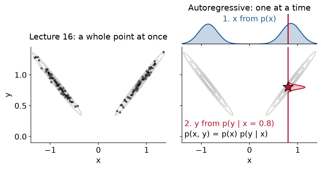
Fig. 130 Lecture 16’s |x| data and its two-component Gaussian mixture, sampled two ways. Left: a whole point at a time, as in Lecture 16. Right: one variable at a time. First \(x\) from the blue curve, \(p(x)\); here \(x = 0.8\). Then \(y\) from the red curve, \(p(y \mid x = 0.8)\), which puts \(y\) near 0.8. Both ways draw from the same distribution.

• Text has too many possibilities to draw at once. A 10-token text has 10 slots, and each slot can hold any of 50,257 tokens, so there are \(50{,}257 \times 50{,}257 \times \dots\) (ten times) \(= 50{,}257^{10} \approx 10^{47}\) possible texts: far too many to list or model directly.

• One token at a time, each step is one choice among 50,257.

The chain rule

• The chain rule of probability writes the probability of a text as a product of next-token probabilities, with no approximation:

\[ \underbrace{p(x_1, \dots, x_T)}_{\text{the whole text}} = \underbrace{\prod_{t=1}^{T}}_{\text{one factor per token}} \underbrace{p(x_t \mid x_1, \dots, x_{t-1})}_{\text{next-token probability}} \]

• The whole text: how likely this exact text is, all \(T\) tokens together.

• One factor per token: multiply the probability of the 1st token, times the 2nd given the 1st, times the 3rd given the first two, and so on to the last.

• Next-token probability: how likely token \(t\) is, given all the tokens before it. This is the only thing an LLM learns.

Example: the chain rule with GPT-2

GPT-2 is a language model OpenAI released in 2019: 124 million parameters, small enough to run on a laptop. We ran it on “The pump stopped” and read its probability for each token, given the ones before it:

\[ p(\text{The pump stopped}) = \underbrace{0.038}_{p(\text{The})} \times \underbrace{8.5 \times 10^{-6}}_{p(\text{␣pump} \mid \text{The})} \times \underbrace{0.0019}_{p(\text{␣stopped} \mid \text{The pump})} = 5.9 \times 10^{-10} \]

• ␣ marks a space: GPT-2’s tokens carry their leading space.

• The product is tiny because so many texts are possible.

• The smallest factor is “␣pump” after “The”, about 8 in a million: thousands of words can follow “The”, and “pump” is a rare one.

• So a model that gives the probability of the next token, from the tokens before it, is a complete generative model of text. It can score a text, and it can write one.

Definition: language model

A language model gives the probability of the next token, \(p(x_t \mid x_1, \dots, x_{t-1})\), from the tokens before it. By the chain rule, that is enough to score a whole text, and to write one. A large language model (LLM) is a language model with billions of parameters, trained on trillions of tokens.

The generation loop

Sampling a text from \(p(x_1, \dots, x_T)\) goes one token at a time:

1. Predict: compute \(p(x_{t+1} \mid x_{\le t})\) for every token in the vocabulary. This is the last factor of the chain rule.

2. Pick: choose one token from that distribution: the most likely one, or a random draw (see Sampling, below).

3. Append it to the end of the text.

4. Repeat from the longer text, until a stop token or a length limit.

We ran GPT-2 on “The pump stopped because the” and, five times, took its most likely next token and appended it:

Step	Text so far	Most likely next tokens	Appended
1	The pump stopped because the	␣water 3.7%, ␣pump 2.9%, ␣gas 2.2%	␣water
2	… because the water	␣was 21%, ␣level 6.5%, ␣had 6.4%	␣was
3	… the water was	␣too 28%, ␣so 5.4%, ␣leaking 4.6%	␣too
4	… the water was too	␣hot 42%, ␣cold 9.9%, ␣high 8.5%	␣hot
5	… the water was too hot	. 35%, ␣and 17%, ␣to 15%	.

• A model that generates this way, each output feeding the next input, is autoregressive.

Autoregressive, as in Lecture 8

• The word is the one from Lecture 8: “Autoregressive models predict the next value as a weighted sum of past values.”

• An LLM does the same with tokens: it predicts the next token from the tokens before it.

• Both make long outputs the same way: feed each prediction back as an input. Lecture 8 called this recursive forecasting; for an LLM it is the generation loop.

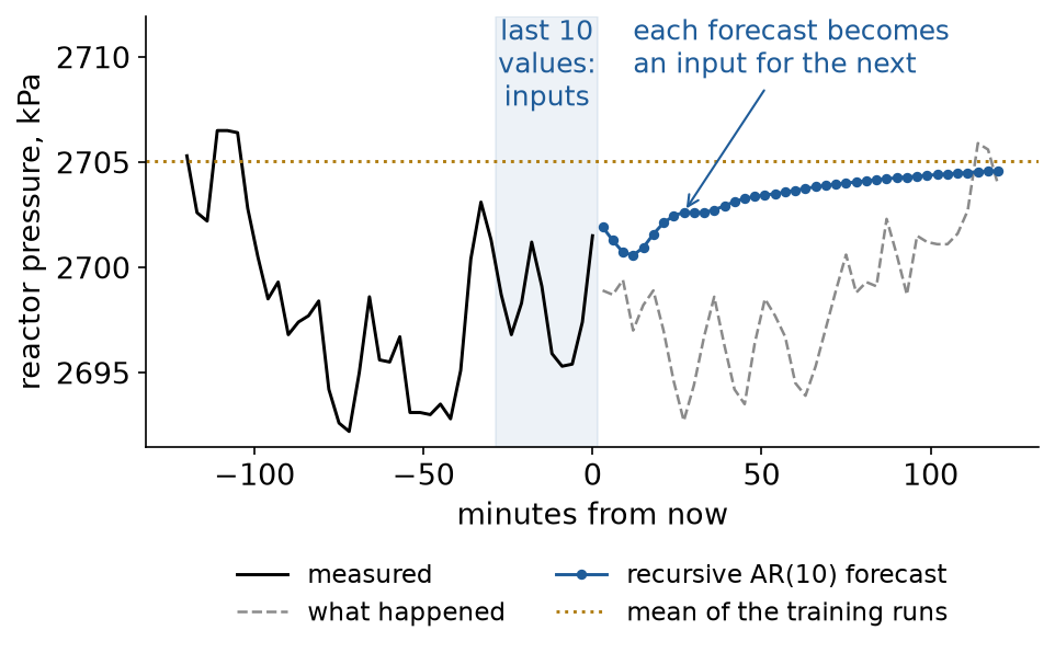
Fig. 131 Lecture 8’s AR(10) on reactor pressure, on one test run (the median of 100 by error), forecast 2 hours ahead. Each blue point was predicted from the 10 before it, most of them earlier forecasts. The forecast drifts toward the training mean while the pressure keeps swinging.

	Lecture 8: AR(10)	An LLM
Predicts	the next pressure	the next token
From	the last 10 values	all the text so far, up to its context window
Output	one number	a probability for every token in the vocabulary
Model	linear, 11 coefficients	a transformer, billions of parameters
Trained	one step ahead, on measured values	one token ahead, on real text
Long outputs	feed each forecast back in	append each token: the same

• The same weakness: both feed their own outputs back in, so an early mistake becomes an input for every later step. In Lecture 8, after two hours the recursive forecast was worse than predicting the mean. In an LLM, one wrong token early in an answer steers every token after it.

• The comparison is between Lecture 8’s forecaster and an LLM. Bengio et al. (2015) saw the same effect in recurrent neural networks, an earlier kind of text generator: trained on true previous tokens and then run on their own, “this discrepancy between training and inference can yield errors that can accumulate quickly along the generated sequence” (Bengio et al., 2015).

Tokens

Definition: token

A token is a piece of text the model reads and writes: a character, a word, or part of a word. The vocabulary is the list of every token the model knows, each with a number, its token id. The tokenizer is the program that cuts text into tokens and looks up their ids.

GPT-2’s tokenizer on one sentence:

Text	The pump stopped.
Tokens	The	␣pump	␣stopped	.
Token ids	464	8901	5025	13

• These are GPT-2’s real ids. Its vocabulary has 50,257 tokens; the model never sees letters, only ids.

• The vocabulary is a lookup table: id 0 is “!”, 13 is “.”, 464 is “The”, 8901 is “␣pump”. The last, 50256, is <|endoftext|>, a special token like the chat tags above: it marks the end of a document.

Three ways to cut a text

“The pump overheated at 85 °C.”, cut three ways:

• Characters: 29 tokens, one per letter, digit, space or symbol. A tiny vocabulary (our tiny GPT has 129), but long sequences: one prediction per character.

• Words: 6 tokens, one per word. Short sequences, but the vocabulary needs every word ever written, and a new one has no token: a pump tag such as P-101A, or a steel grade such as AISI 4140.

• Subwords: pieces of words. GPT-2 needs 9 tokens here: The | ␣pump | ␣overhe | ated | ␣at | ␣85 | ␣° | C | .. Common words stay whole (”␣pump”), rarer ones split (”␣overhe” + “ated”), so any new word can still be built. This is what LLMs use: GPT-2 has 50,257 tokens, GPT-4o about 200,000.

Byte-pair encoding

Definition: byte-pair encoding

Byte-pair encoding (BPE) is how a subword vocabulary is built. Find the pair of neighboring tokens that appears most often, merge it into one new token, repeat (Sennrich et al., 2016).

Wikipedia’s example (Byte-pair encoding), on the text “aaabdaaabac”:

Step	Most frequent pair	Tokens	Count
start		a a a b d a a a b a c	11
1	a + a (4 times)	aa a b d aa a b a c	9
2	a + b (2 times)	aa ab d aa ab a c	7
3	aa + ab (2 times)	aaab d aaab a c	5

• Step 2 is a tie: “aa” + “a” also appears twice. Wikipedia’s example takes “a” + “b”.

Why this is useful:

• Fewer tokens. Frequent pieces become one token, so sequences get shorter: more text fits in the context window, and writing it takes fewer steps.

• Nothing is unknown. A new word can always be built from smaller pieces, down to single characters; GPT-2 starts from bytes, so it can write any text.

• Learned from data. The merges come from the training text, so its frequent words become single tokens. A tokenizer learns its merges once and applies them, in order, to any new text.

The algorithm is Philip Gage’s, a data-compression method from 1994, adapted to building subword vocabularies by Sennrich et al. (2016). GPT-2 starts from bytes and stops after 50,000 merges.

Byte-pair encoding learned from our notes

• We learned 600 merges by BPE from our notes (Lectures 1 to 16), then applied them, in order, to one sentence. Press play to watch the merges.

• The last row is GPT-4o’s tokenizer, learned the same way from far more text and loaded with OpenAI’s tiktoken library.

• Each merge makes tokens longer and fewer. 35 characters become 18 tokens with our 600 merges, and 10 with GPT-4o’s tokenizer.

• Fewer tokens means more text fits in the context window, and writing it takes fewer steps.

Numbers and units cost more than words

• Common words are one token each. Numbers, units, part numbers and formulas split into many.

• Same length, very different cost: “heat exchanger” is 14 characters and 2 tokens. “Q = 1.5e-3 m³/s” is 15 characters and 12 tokens.

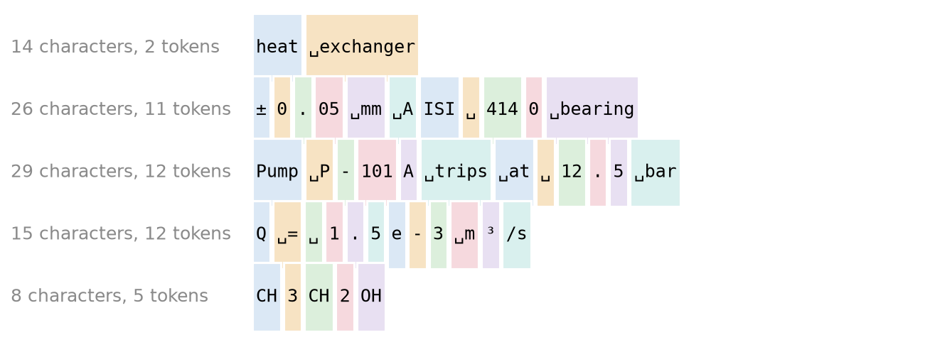
Fig. 132 Each box is one token of GPT-4o’s tokenizer (o200k_base, in tiktoken); the left column gives characters and tokens per string. Words cost one token; numbers and symbols cost one token every few characters. “AISI” becomes “ A” and “ISI”, and “4140” becomes “414” and “0”.

• The model reads numbers in pieces. The tokenizer cuts “4140” (the steel grade in the figure) into two tokens, “414” and “0”, the way it cuts a word into pieces, and “12.5” into “12”, “.” and “5”. The model sees text pieces, never the quantity four thousand one hundred forty. P-101A in the figure is a pump tag; it splits the same way.

• So numbers, units and part numbers are where LLMs slip. Check them, and do the arithmetic in code.

The context window

Definition: context window

The context window is the most tokens a model can take in at once: your prompt, any documents, and everything it has written so far.

• Our tiny GPT: 128 characters, about one sentence.

• GPT-3: “a context window of nctx = 2048 tokens”, a few pages (Brown et al., 2020).

• Llama 3: “a context window of up to 128K tokens”, a long report (Llama Team, 2024).

• Our notes of Lectures 1 to 16 are 164,779 tokens with GPT-4o’s tokenizer: they do not fit in a 128,000-token window.

• Text beyond the window is not seen at all. Long documents must be cut, summarized or searched.

• Cost and time are counted in tokens, so the context window is a budget.

The model: a transformer that only looks back

The big picture

• We gave GPT-2 the prompt “The plant shut down for maintenance” and asked for the next token.

• Watch “plant”: on its own, it could be a tree or a factory. Press play.

• The final probabilities are GPT-2’s; the vectors and the meaning map are a sketch.

1. Tokens become vectors: each token becomes a list of numbers. On its own, “plant” could be a tree or a factory.

2. Attention: each vector takes information from the ones before it. “plant” reads “shut down” and “maintenance” and moves toward “factory”.

3. MLP: each vector is then updated on its own, by the same small network.

4. Repeat: attention, then MLP, 4 times in our tiny GPT and 96 times in GPT-3.

5. The last vector gives the next token. GPT-2’s top guess is “␣in”, 19%, as in “…for maintenance in March”.

• This is the transformer of Lecture 12, where the tokens were cycles of a sensor window. The machinery is the same.

Attention looks back

• One change from Lecture 12: a token may attend only to itself and the tokens before it.

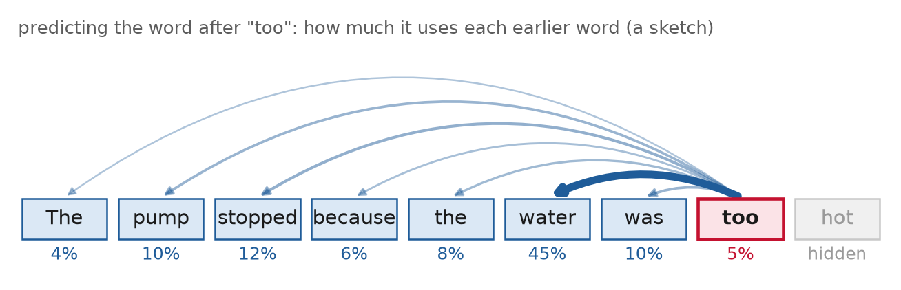
Fig. 133 A sketch of attention when the model predicts the word after “too”: it looks back at every earlier word and uses “water” most. The weights are illustrative. The next word, “hot”, is hidden by the causal mask: in training it is the answer.

1. Score: the word “too” asks every earlier word: how useful are you for guessing what comes next?

2. Mix: it takes a weighted average of what those words carry. Here, mostly “water”.

3. No peeking: later words are hidden, by the causal mask. In training the next word is the answer, so it must stay hidden.

In symbols, as in Lecture 12:

\[ \mathrm{softmax}\Big(\frac{QK^\top}{\sqrt{d_k}} + M\Big)\, V \]

• \(QK^\top/\sqrt{d_k}\) are the scores. The mask \(M\) is \(-\infty\) for later words, which sets their weight to 0.

Definition: causal mask

A causal mask stops each position from attending to later positions, so the prediction at position \(t\) uses only tokens \(1\) to \(t\).

• A transformer with only this masked attention is decoder-only. GPT-2, GPT-3, Llama and our tiny GPT are all decoder-only.

Training: predict the next token, everywhere

Tuning the dials

• The model’s behavior is set by its parameters, like the dials of a machine. A straight-line fit in Lecture 9 has 2; our tiny GPT has 842,881; GPT-3 has 175 billion. They start random, so the model writes gibberish.

• One training step: show the model some text with the next character hidden; it guesses; compare its guess with the true character; nudge every dial a little so the true one gets more likely. Repeat, 2,000 times for our tiny GPT.

• The nudge is a gradient step. Backpropagation, the automatic differentiation of Lecture 11, gives the gradient for every dial in one backward pass.

• Below, our tiny GPT on one example, “…learns the proba?”. The true answer is “b”. Press play.

• It gives “b” 0.4% before training, 48% at step 750, and over 99% at step 2,000.

• The dials are a drawing. The guesses and the chart are the tiny GPT’s own, saved every 250 steps.

The objective

• Training makes real text likely. By the chain rule, a text’s log-probability is a sum over its tokens. We want it large, so we minimize its negative, averaged per token.

Definition: pretraining

Pretraining fits a language model to a large body of text by minimizing the next-token cross-entropy: the average of \(-\log p\) of the token that actually came next.

\[ \mathcal{L}(\theta) = \underbrace{-\frac{1}{T} \sum_{t=1}^{T}}_{\text{minus, averaged}} \underbrace{\log p_\theta(x_{t+1} \mid x_1, \dots, x_t)}_{\text{log probability of the true next token}} \]

• \(\theta\): the parameters, the dials. \(p_\theta\) is the model with those parameters.

• Log probability of the true next token: how much probability the model gave the token that really came next.

• The minus: it makes the quantity a loss to minimize. The loss of one prediction, \(-\ln p\), is 0 when the model gave the true token probability 1, 0.69 for a coin flip (\(p = 0.5\)), and 4.86 for a blind guess among 129 characters.

• The average: \(\frac{1}{T}\sum_t\) averages over the \(T\) positions, so the loss is per token.

• Cross-entropy: each position is a classification over the vocabulary, as in Lecture 10.

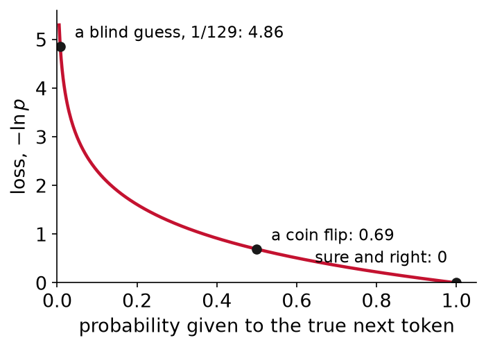
Fig. 134 The loss of one prediction. Being right and sure costs nothing; being surprised costs a lot.

Every position at once

• Below, one sentence of 10 tokens turned into 9 guesses. Guess 1: from “The” alone, guess the next token. Guess 2: from “The pump”. Press play.

• Self-supervised: the labels are the text itself, shifted by one. No one labels anything, which is why trillions of tokens are usable.

• Every position at once: one sentence gives 9 training examples, all done in one pass.

• Each guess sees only the tokens before it, because of the causal mask. Without it, the answer would be in plain sight.

Training is an optimization problem

\[ \min_{\theta}\;\; \mathcal{L}(\theta) = -\frac{1}{N} \sum_{n=1}^{N} \log p_\theta\big(\text{next token}_n \mid \text{the tokens before it}\big) \]

• Decision variables: the parameters \(\theta\): 842,881 in our tiny GPT, 175 billion in GPT-3.

• Objective: the loss over all \(N\) predictions, the same kind of data loss as the \(\min_\theta L_\text{data}\) of Lecture 13.

• Method: gradient-based. Backpropagation gives \(\nabla_\theta \mathcal{L}\) in one backward pass, and AdamW (Lecture 12) takes the step. The large models do the same: GPT-3 was trained with “Adam with β1 = 0.9, β2 = 0.95” (Brown et al., 2020), and Llama 3 405B “using AdamW” (Llama Team, 2024).

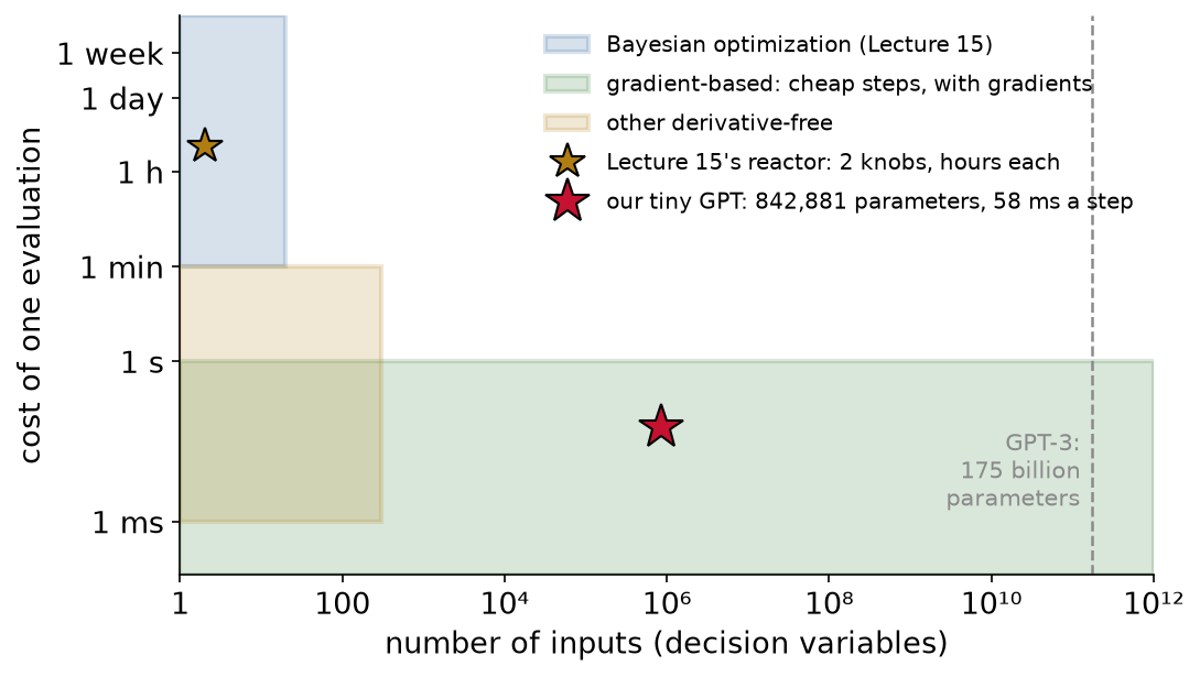
Fig. 135 Lecture 15’s map of where each optimizer fits, with our tiny GPT added. The reactor (gold star) has 2 knobs and hours per experiment: Bayesian optimization. The tiny GPT (red star) has 842,881 knobs and 58 ms per training step, with gradients: gradient descent.

Reading the loss

• At the start, the dials are random: each of the 129 characters gets about the same chance, 1/129. A model that knows nothing has a loss of \(-\ln(1/129) = \ln 129\). With our 129 characters, that is 4.86. Our tiny GPT’s first loss was 4.67, near 4.86.

• To read a loss, undo the \(\ln\). The loss is the average of \(-\ln p\), so \(e^{-\text{loss}}\) is the typical \(p\) (the geometric mean). Our tiny GPT reaches 1.51 on held-out text after 2,000 steps, and \(e^{-1.51} = 0.22\): on text it never saw, it typically gives the right next character a 22% chance.

Loss	Typical \(p = e^{-\text{loss}}\)
4.86	0.8%	a blind guess, 1/129
1.51	22%	our tiny GPT at the end, on held-out text
0.69	50%	a coin flip
0	100%	sure and right

• “Typical” is not the share of right guesses: it is the geometric mean of the probabilities the model gave the true characters.

• Equivalently, \(e^{1.51} \approx 4.5\): the model is about as unsure as a choice among 4.5 equally likely characters, instead of 129.

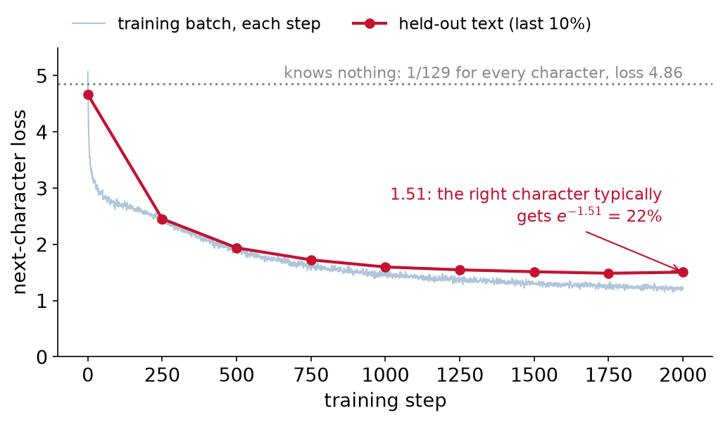
Fig. 136 Our tiny GPT over 2,000 training steps. Blue: the loss on each training batch. Red: the loss on the last 10% of the notes, never trained on. Dotted: a model that knows nothing. Both curves drop fastest in the first 500 steps; the red one levels off while the blue one keeps falling.

• Its training loss (1.22) falls below its held-out loss (1.51): with 0.6 million characters, it starts to memorize. This is the overfitting of Lecture 9; the held-out curve is the one to trust.

What it writes as it learns

What the tiny GPT writes after “The model “, at temperature 0.8, as training goes on:

Step	Held-out loss	It writes	What changed
0	4.67	The model l₂4zé'-(u↑Ly°⁷)aQ8d¹₆−wZ²t,>zü4i{₂YG	random characters
250	2.46	The model 100.5 06 ` dastand and the gry lenpt.	letters, spaces, line breaks; almost no words
500	1.94	The model is onlow you be column is a sque, and with the defforemation	short real words, glued into nonsense
1,250	1.55	The model windows where the forecaster is the residual.	phrases from the course
2,000	1.51	The model of the data, and in a \text{sk}} = \underbrace{\frac{dX}{dt}	LaTeX copied from our notes

• Spelling, words and Markdown come first. Meaning comes much later, and with far more data.

• It learned only from our notes, so it copies their style, LaTeX included. Far more text, and a bigger model, are what turn style into meaning.

What our tiny GPT learned

A test with a fixed rule: take one term from each of Lectures 1 to 16, give the model the first 60% of its characters, and let it pick the most likely next character until the term ends.

Lecture	Given	Finished		Lecture	Given	Finished
1	toolch	ain ✓		9	regres	sion ✓
2	environ	ment ✓		10	classific	ation ✓
3	datab	ase ✓		11	gradi	ent ✓
4	Parqu	et ✓		12	convolu	tion ✓
5	datafr	ame ✓		13	physics-in	to a s ✗
6	valida	tion ✓		14	uncerta	inty ✓
7	steady s	tate ✓		15	Bayesian opti	mization ✓
8	forec	ast ✓		16	distribu	tion ✓

• 15 of 16 right: it learned our spelling and our vocabulary.

• The miss is a frequency effect: “into a” appears 58 times in our notes, “physics-informed” only 8.

• No sentences with meaning: asked to go on, it writes “and the same step of the same samples”. Meaning takes far more parameters and data: the next section.

Data and scale

Models over the years

• Language models by year and size, on a log scale: each labeled line is 1,000 times the one below. Press play.

• Closed models publish no size: they sit on the strip at the top.

• Published sizes grew fast: GPT-1 had 117 million parameters (2018), GPT-2 1.5 billion (2019), GPT-3 175 billion (2020) and PaLM 540 billion (2022).

• Recent open models are mixtures of experts: they use only part of their parameters for each token (the hollow dots). DeepSeek-V3 has 671 billion with 37 billion active (2024); Kimi K3 has 2.8 trillion with 104 billion active (2026).

• Sources: GPT-1 and GPT-2, GPT-3, PaLM, DeepSeek-V3, Kimi K3.

• Closed models publish no size. The GPT-4 report “contains no further details about the architecture (including model size)” (OpenAI, 2023); nor do later GPT models (GPT-6 Astra, September 2026) or Anthropic’s Claude models.

In human terms

• Their data: mostly filtered web text, plus books, code and papers. Llama 3 used “about 15T multilingual tokens.”

• Our data: the notes of Lectures 1 to 16, 668,651 characters. In 2,000 steps the tiny GPT sees each character about 27 times.

• Reading it: our notes take about 7 hours to read, at 250 words a minute. Our notes run at 0.58 words per GPT-2 token, and GPT-3 uses the same vocabulary, so its 300 billion training tokens would take about 1,300 years of non-stop reading.

• Computing it: training costs about 6 operations per parameter per token: about 8 × 10¹³ for our tiny GPT. A laptop GPU did that in 2 minutes, about 700 billion operations a second; at one billion a second it would take about 23 hours. GPT-3 needed 3.14 × 10²³ (Brown et al., 2020, Table D.1): about 10 million years at a billion a second.

After pretraining

A chat model is made in three stages:

1. Pretraining: the model learns to continue text, from trillions of tokens. We gave GPT-2 “What is the boiling point of water?”, and it continued “The boiling point of water is the point at which the water boils.”, then repeated that sentence.

2. Supervised fine-tuning (SFT) trains it further, with the same next-token loss, on examples of instructions and good answers, written by people. InstructGPT “hired a team of about 40 contractors” to write them and to rank answers (Ouyang et al., 2022).

3. Preference tuning: people pick the better of two answers, and the model learns their preference, by one of two methods:

   • Reinforcement learning from human feedback (RLHF): a reward model learns their picks, and the LLM is tuned to score high on it.

   • Direct preference optimization (DPO): the same picks, used directly: “without explicit reward modeling or reinforcement learning” (Rafailov et al., 2023).

• The result is a chat model: the same network, now answering. Qwen2.5-0.5B-Instruct, from the opening example, answers “In one sentence, what does a heat exchanger do?” with “A heat exchanger transfers heat from one medium to another.”

• Still how it is done: in Llama 3, “each round of post-training involves supervised finetuning (SFT) followed by Direct Preference Optimization (DPO; Rafailov et al., 2024) on examples collected either via human annotations or generated synthetically” (Llama Team, 2024).

• Pretraining gives the knowledge and the fluency, from trillions of unlabeled tokens. Post-training changes the behavior, with far less data written or ranked by people. The chat model still completes a script: the hidden script of the opening example.

Sampling: temperature

Definition: temperature

Temperature \(\tau\) is a knob for how adventurous the model is when it picks the next token. Low: it almost always takes the most likely token. High: less likely tokens get a real chance.

\[ p_\tau(v) = \frac{e^{z_v / \tau}}{\sum_{u \in \text{vocabulary}} e^{z_u / \tau}} \]

• \(z\): the logits, the model’s raw score for each token, before the softmax turns them into probabilities. Higher means more likely.

• \(\tau\) (tau): divide every logit by \(\tau\), then take the softmax. Below 1, it sharpens the distribution toward the most likely token; above 1, it flattens it. At \(\tau = 1\), these are the model’s own probabilities.

• Example, two logits, 2 and 1: at \(\tau = 1\), 73% and 27%. At \(\tau = 0.5\) the gap doubles: 88% and 12%. At \(\tau = 2\) it halves: 62% and 38%.

• “Using a higher value for T produces a softer probability distribution over classes” (Hinton, Vinyals and Dean, 2015).

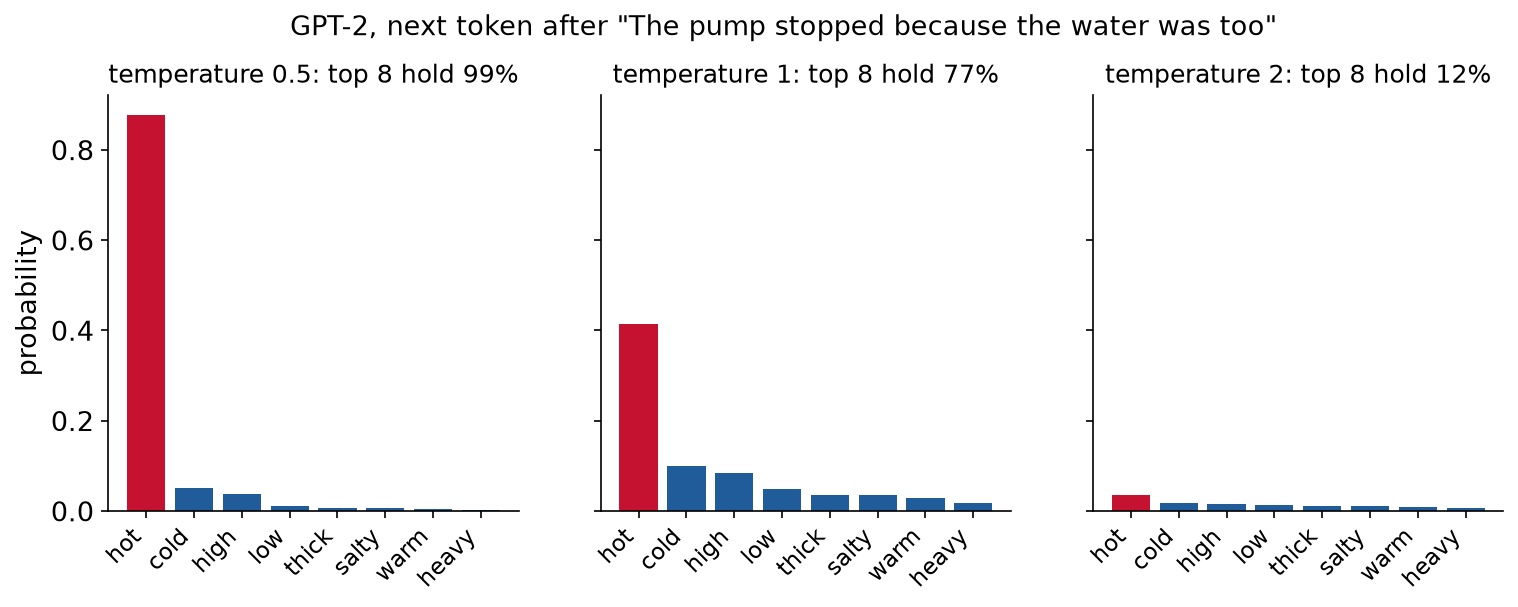
Fig. 137 We ran GPT-2 on “The pump stopped because the water was too” and applied three temperatures to its logits, over its whole vocabulary of 50,257 tokens. “␣hot” gets 88% at temperature 0.5, 42% at 1 and 4% at 2. The red bar is the most likely token.

• \(\tau \to 0\): always the most likely token (greedy decoding). Repeatable, often repetitive.

• \(\tau = 1\): the model’s own probabilities.

• \(\tau > 1\): unlikely tokens get a real chance. More varied, more mistakes.

Spin the wheel

• Sampling is spinning a wheel with one slice per token, sized by its probability. Below, GPT-2’s next token after “…the water was too”. Change \(\tau\), then spin.

• \(\tau\) changes the wheel; the spin stays fair. At \(\tau = 0.5\), “␣hot” takes 88% of the wheel; at \(\tau = 2\), only 4%.

• Why “temperature”: the softmax with a temperature is Boltzmann’s distribution from thermodynamics:

\[ p(\text{token } v) = \frac{e^{z_v/\tau}}{\sum_u e^{z_u/\tau}} \qquad\qquad p(\text{state } i) = \frac{e^{-E_i/k_BT}}{\sum_j e^{-E_j/k_BT}} \]

• A logit \(z\) plays minus an energy, and \(\tau\) plays \(k_BT\). Hot: every state gets visited. Cold: the lowest-energy state wins.

• “In statistical mechanics, the softmax function is known as the Boltzmann distribution” (Wikipedia, after LeCun et al., 2006).

The loop with a temperature knob

• Below, GPT-2’s ten most likely next tokens at each step of the generation loop. Red: the one appended. Step through, then move \(\tau\).

• \(\tau = 1\): GPT-2’s own probabilities. At step 1, “␣water” gets 3.7%: many words could follow.

• \(\tau = 0.1\): “␣water” jumps to 89%. Low temperature gives nearly the same text every time.

• \(\tau = 2\): every bar flattens. At step 4, even “␣hot” falls to 4%: almost anything can come next.

Our tiny GPT at three temperatures

From the same prompt, “A Gaussian process”, and the same model; only \(\tau\) changed:

• \(\tau = 0.3\): “… a strain of the same data is the same offf the same way”: safe and repetitive, with a Markdown heading copied from our notes.

• \(\tau = 0.8\): “… the default does not exact the band file coefficients the wide, vector plant”: varied words in our style, with no meaning.

• \(\tau = 1.5\): “… cructor arNive,” and a brieful mini-bassed flrecash”: broken words and rare symbols, the tail of the distribution.

Fluent is not the same as true

Definition: hallucination

A hallucination is fluent, confident text that is false: an invented number, unit, citation or fact.

• A chat model: we ran Qwen2.5-0.5B-Instruct (0.49 billion parameters, trained on 18 trillion tokens) on a laptop and asked “What is the boiling point of water at sea level?”. It answered “The boiling point of water at sea level is 100 degrees Fahrenheit.”

• After “…100 degrees” it gave “␣Fahrenheit” 58.6% and “␣Celsius” 40.8%, and took the more likely one. The number is right; the unit is a near coin flip.

• A pretrained model: given “Question: What is the boiling point of water at sea level? Answer:”, GPT-2 writes “The boiling point of water at sea level is about 1,000 degrees Fahrenheit.” The true value is 212 °F (100 °C).

• Why: pretraining rewards the likely next token. Nothing in the loss checks a fact.

• Larger models and post-training make this rarer. They do not remove it.

• So: treat every number and unit from an LLM as unchecked. Check it against a measurement, a handbook or a calculation.

Limitations and trade-offs

• It invents sources and software packages. In code from GPT-3.5, GPT-4 and GPT-4 Turbo, “the average percentage of hallucinated packages is at least 5.2%”, and 21.7% for open models (Spracklen et al., 2025). Attackers can publish malicious code under an invented name. Check that each source and package exists before you cite or install it.

• Coding agents act on their guesses: they edit files, install packages and run commands. Review the diff and run the tests before you merge, and keep secrets out of their reach.

• It knows only its training data: nothing after its cutoff date, and nothing in your company’s documents. Put the documents it needs in the prompt, and do not ask it for current values.

• Long inputs: answers get worse as inputs grow, well inside the advertised window (Hsieh et al., 2024; Du et al., 2025). Facts in the middle of a long input used to be the worst served (Liu et al., 2024); newer models show that less, but the drop with length remains. Send only what matters: retrieve the relevant parts, ask the model to quote its evidence, and repeat the main instructions.

• Numbers and units: the model reads 4140 as two text pieces, “414” and “0”, never as a quantity. It predicts digits as tokens; it does not calculate. Do arithmetic and unit conversions in code.

• It is not reproducible: the same prompt can give another answer, even at temperature 0. Save the output you used, with the model’s name and the date, as in Lecture 1.

• Your prompt leaves your machine for the provider’s servers. Check your company’s rules before you paste its data, or run an open model locally.

Summary

An LLM is a generative model of text. The chain rule turns the probability of a text into a product of next-token probabilities, so a model that predicts the next token, from the tokens before it, can both score text and generate it, one token at a time. Generation is Lecture 8’s recursive forecast with tokens instead of pressures, and it shares its weakness: errors feed forward. The tokens come from byte-pair encoding, which is why common words are cheap and part numbers, units and formulas are not. The model is the transformer of Lecture 12 with a causal mask, and pretraining minimizes the next-token cross-entropy at every position of every context window, by gradient descent on billions of parameters. The same loop, on 0.6 million characters of our notes, gives a model that spells like the course and means nothing; meaning takes far more text and a far bigger model. Post-training turns a model that continues text into one that answers. Temperature sets how adventurous the sampling is. Nothing in the loss checks a fact, so every number an LLM gives you needs checking.

Resources

With thanks to 3Blue1Brown

This lecture is built on Grant Sanderson’s lessons on large language models (text adaptations by Justin Sun), the clearest visual explanation of them we know. The chatbot as a script it completes, training as tuning dials, vectors that talk to each other, and temperature all come from there. Watch them before anything else on this list.

• Large Language Models explained briefly (video, 2024, about 8 min). The whole idea in one sitting: next-word prediction, training as tuning dials, pretraining and RLHF, attention.

• Transformers, the tech behind LLMs (video, Chapter 5). The structure of the model, embeddings as directions with meaning, softmax and temperature.

• Attention in transformers, step-by-step and How might LLMs store facts (Chapters 6 and 7). Attention and the MLP, in depth.

Videos

• Karpathy, Intro to Large Language Models (2023, 1 h). Pretraining, fine-tuning and what comes next, for a general audience.

• Karpathy, Let’s build GPT: from scratch, in code, spelled out (2023, 2 h). How a tiny GPT like ours is built, in code.

• Karpathy, Let’s build the GPT Tokenizer (2024, 2 h). Byte-pair encoding, in code.

• Karpathy, Deep Dive into LLMs like ChatGPT (2025, 3.5 h). The full pipeline, from data to chat model.

Interactive

• Transformer Explainer. GPT-2 running in your browser: type a prompt, step through the layers, move the temperature.

• LLM Visualization. A 3D walk through every computation of a small GPT.

• Tiktokenizer. Paste text, see the tokens and the count.

Reading

• Alammar, The Illustrated GPT-2. Masked self-attention and generation, in pictures.

• Jurafsky and Martin, Speech and Language Processing, 3rd ed. draft, free online: Chapter 2 (tokens and BPE), Chapter 7 (transformers and pretraining), Chapter 8 (post-training).

• Hugging Face LLM Course. Free, hands-on, with the transformers library.

• Papers: GPT-3 (Brown et al., 2020), InstructGPT (Ouyang et al., 2022), DPO (Rafailov et al., 2023), Llama 3 (Llama Team, 2024).

Assignment

No assignment is released with this lecture. The final project is released today: team agreement due Friday 10-30, proposal due Wednesday 11-04.

Practice module

Practice module for this session, for participation credit.