Lecture 12: Architectures for engineering data: MLP, CNN, and sequence models#
Overview
Session Lecture 12, Week 6
Arc Machine learning and deep learning
Slides Deck for this session
Practice Practice module for this session
Demo
l12-cnn-rul.ipynb, a 1D-CNN for turbofan remaining-useful-life, against a tabular baselineAssignment 6, released at Lecture 11; this session’s architectures are what it asks you to build
Why this matters#
Lecture 11 built the machinery: tensors, autograd, a training loop, and a multilayer perceptron on tabular concrete data. It also delivered an occasionally awkward result, that the MLP did not beat a gradient-boosted tree. This session is about the missing idea that a bare MLP throws away, which is structure.
An MLP treats its input as a flat vector of numbers with no relationships among them. That is the right picture for tabular data, where the columns are genuinely different quantities. It is the wrong picture for a great deal of engineering data, where the input has a shape the model should exploit. A temperature field from a simulation is a grid, and a pixel’s neighbors matter. A vibration trace is a sequence, and a reading’s recent past matters. Flatten either into a vector and you have told the model to relearn, from scratch and from limited data, a structure you already knew for free.
Matching the architecture to that structure is the whole subject. A vector goes to an MLP. A field or an image goes to a convolutional network. A sensor time series goes to a one-dimensional convolution or a recurrent network. The payoff is a model with fewer parameters that generalizes better, because it builds in an assumption that happens to be true. The honest counterweight, which this session takes as seriously as the promise, is that a deep architecture is not a default: on the turbofan data below, a quick 1D-CNN does not beat a well-built tabular baseline, and the reason it does not is as instructive as the cases where it does.
Learning objectives#
By the end of this session you should be able to:
Match model architecture to the structure of the input (vector, field/image, sequence).
Implement a 1D-CNN or RNN for sensor time series and a 2D-CNN for field/image data.
Apply regularization and normalization appropriate to each architecture.
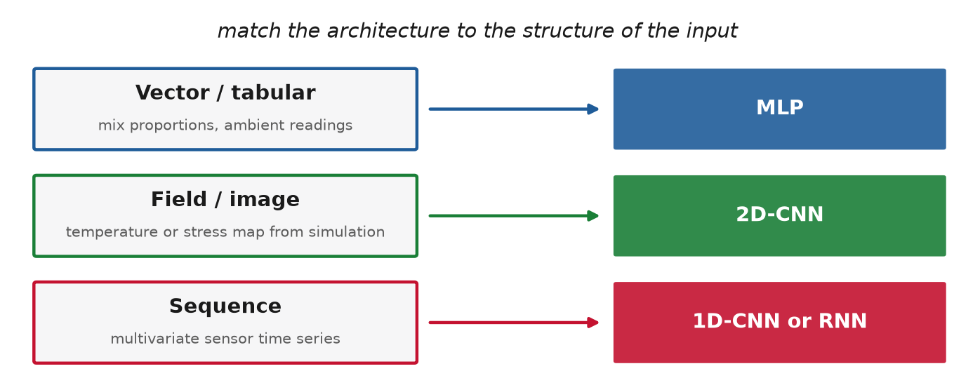
Fig. 73 The one decision this session is about. The structure of the input, not the size of the dataset or the fashion of the method, is what should pick the architecture.#
MLPs, and why scaling still matters#
The multilayer perceptron is the architecture for vector inputs, and Lecture 11 built one, so this session only adds the choices that shape it. Its two dials are width (units per layer) and depth (number of layers); more of either adds capacity and, past the point the data can constrain, adds overfitting. Between layers sits a nonlinear activation, and the modern default is ReLU (or its smoother cousin GELU), which trains faster than the older saturating sigmoids and tanh. Three regularizers keep a wide MLP honest: dropout, which randomly zeros a fraction of activations during training so the network cannot lean on any single unit; weight decay, which penalizes large weights; and batch or layer normalization, which rescales activations to keep the gradients well behaved.
One habit from earlier weeks does not go away because the model is now a neural network. Feature scaling still matters, because gradient descent on unscaled inputs takes tiny steps along the large-range features and overshoots the small-range ones. Lecture 11 measured the cost: unnormalized inputs make plain SGD produce a nan in the first epoch, while Adam quietly trains to a mediocre score and reports nothing wrong. Fold the scaler into the pipeline and fit it on training data only, exactly as in Lecture 7, because a neural network does not repeal the leakage rules from the Data Systems arc.
CNNs for fields and images#
A convolutional network is the architecture for data laid out on a grid: an image, or an engineering field such as a temperature, stress, or velocity map from a simulation. Its core operation is convolution, sliding a small kernel (a grid of weights, perhaps 3 by 3) across the input and computing a weighted sum at each position to produce a feature map. A few terms describe the sliding: the stride is how far the kernel moves between positions, padding adds a border so the output can keep the input’s size, and channels are the stacked feature maps (three for a color image, one for a scalar field, many inside the network). Pooling then downsamples a feature map, taking the maximum or average over small regions, so deeper layers see a coarser, larger view.
The figure below runs each of these operations on an 8 by 8 temperature field with one hot spot, small enough that every number can be checked by hand. Under kernel, press Play and follow the box: each output is the nine products of kernel weight and temperature, summed, and the same nine weights produce all 36 outputs. The vertical-edge kernel responds where temperature changes from left to right, positive on the rising side of the hot spot and negative on the falling side. Under stride and padding, the readout gives the output size, \(\lfloor (n + 2p - k)/s \rfloor + 1\), for the settings you choose: stride 2 roughly halves each side, and one ring of zero padding lets the kernel center on the edge cells. Under channels, three kernels read the same input and write three maps, which the next layer takes as a three-channel input, so its kernels are 3 by 3 by 3. Engineering inputs often start with several channels: a CFD snapshot carrying velocity components, pressure, and temperature is a four-channel image. Under pooling, a 2 by 2 window with stride 2 keeps the maximum or the mean of each block and learns nothing, which cuts the map to a quarter of its values and doubles the reach of every kernel that follows.
Definition: convolution and the receptive field
A convolution applies the same small kernel of weights at every position of the input, so a feature learned in one place is detected everywhere. The receptive field of a unit is, in the words of Stanford’s CS231n, “the spatial extent of this connectivity … equivalently this is the filter size”: the region of the input that can influence it. Stacking convolutions and pooling grows the receptive field, so deep units see wide context from small kernels.
Two properties explain why a CNN needs far fewer parameters than an MLP for the same grid. Goodfellow, Bengio, and Courville put it that “convolution leverages three important ideas: sparse interactions, parameter sharing and equivariant representations.” Sparse interactions come from the kernel being smaller than the input, so each output depends on a small patch rather than every input pixel. Parameter sharing means “using the same parameter for more than one function in a model”: the same kernel weights are reused at every position, because a feature worth detecting in one corner of an image is worth detecting in the others. An MLP with a weight per input-output pair would have to learn each position’s edge detector separately, from far more data. On the 8 by 8 field in the figure above, the convolution uses 9 weights for all 36 outputs, while a dense layer mapping the same 64 inputs to 36 outputs needs 64 × 36 = 2,304. That reuse is why a CNN, not a bigger MLP, is the right tool for a stress field.
The kernels will look familiar to anyone who has discretized a PDE. The vertical-edge kernel in the figure, with columns of −1, 0, and +1, is a central-difference stencil for \(\partial T / \partial x\), summed over three neighboring rows; image processing calls it the Prewitt operator, one of a pair of 3 by 3 kernels that approximate the horizontal and vertical derivatives. A convolutional layer is a bank of such stencils whose coefficients are learned from data instead of derived from a Taylor expansion.
Sequence models for sensor time series#
A sensor time series is a grid in one dimension, time, with a channel per sensor. Two architectures exploit that shape.
A 1D convolution slides a kernel along time instead of across space. torch.nn.Conv1d, in the docs’ words, “applies a 1D convolution over an input signal composed of several input planes,” the planes here being the sensor channels. A 1D-CNN learns local temporal patterns (a spike, a ramp, a change in variance) and, stacked, assembles them into longer-range features, with the same parameter-sharing economy as its 2D cousin.
The figure below slides one kernel along a real engine, sensor 11 of FD001 engine 1 over its last 60 cycles before failure. Step it with the least-squares slope kernel and the output rises as the engine approaches failure, because a slope kernel is exactly a local trend detector. Switch to the average kernel and the same machinery smooths the noise instead, and the random kernel shows what a network starts from before training chooses the weights.
Stacking layers is how a convolution sees further than its kernel. Each layer adds \(k-1\) cycles of reach, so three layers of width-5 kernels give one output a receptive field of \(1 + 3 \times 4 = 13\) cycles, less than half of a 30-cycle window. The figure also shows a cost of “same” padding that is easy to miss: the output at the last cycle is centred on the window’s edge, so six of its thirteen inputs are padding zeros and only seven are data. Dilating the layers by 1, 2 and 4 widens the reach to 29 cycles with the same number of weights, which is the idea behind the temporal convolutional network.
A recurrent network instead walks the sequence step by step, carrying a hidden state that summarizes the past. Plain RNNs struggle to remember far back, so the practical variants are the LSTM and GRU, which add gates that let the state retain information over long spans; torch.nn.LSTM “applies a multi-layer long short-term memory (LSTM) RNN to an input sequence.”
The figure below shows the recurrence at its simplest, one state unit with its update gate held fixed. At each cycle the new state is a blend of the old state and the new input, \(h_t = (1-z)\,h_{t-1} + z\,x_t\), and the prediction reads only the final state. A small \(z\) gives a long, smooth memory of roughly \(1/z\) cycles, and \(z = 1\) forgets everything but the latest input. A GRU learns \(z\) and computes it from the input at every step, which lets it decide when to hold its summary and when to overwrite it.
The same chain explains why plain RNNs forget. Training propagates the loss back through the recurrence one step at a time, multiplying by roughly the same factor at each step, so the signal reaching cycle 1 of a 30-cycle window is that factor raised to the 29th power. Below 1 it vanishes geometrically, and above 1 it explodes, which is the problem Bengio, Simard and Frasconi analysed in 1994. Gradient clipping rescales an exploding gradient, but no rescaling recovers one that has vanished. The GRU’s gate is the fix for that, because its state path multiplies by \((1-z)\), which training can hold close to 1.
Which to reach for is a genuine engineering choice, and the answer has shifted. For years the reflex was an RNN for anything sequential, but Bai, Kolter, and Koltun (2018) found that “a simple convolutional architecture outperforms canonical recurrent networks such as LSTMs across a diverse range of tasks and datasets.” A temporal CNN trains faster (its timesteps compute in parallel, where an RNN must go in order), handles short-to-medium windows well, and is the sensible default for the fixed-length sliding windows a sensor feed produces. Reach for an LSTM or a GRU when the dependence is genuinely long-range and variable. The third family, attention and the transformer, gets its own section below, because it makes the fewest assumptions of the three and that changes how it behaves on a dataset this size. Whatever the architecture, the windows must be normalized with statistics fit on training data only, and windowed so that no window straddles two units, which is the leakage lesson from Lecture 8 arriving in a new shape.
The four architectures differ most visibly in their wiring, meaning which cycles can influence which hidden units and whether the weights are shared across time. The figure draws one hidden layer over a short window for each. The MLP connects everything with separate weights, the CNN connects only neighbours through shared weights, the GRU passes a single shared update along a chain, and the transformer connects every cycle to every other with weights computed from the data itself.
Attention and transformers for sequences#
The third way to read a window is to let every cycle look at every other cycle directly, and to decide from the data how much each one matters. A convolution reads a few neighbours with fixed weights. A GRU reads the past only through its one state vector, which has to carry everything forward. Self-attention lets cycle 30 read cycle 3 in a single step, with a weight computed from what the two cycles contain. Vaswani and colleagues built the transformer around this operation in 2017, describing it as “a new simple network architecture, the Transformer, based solely on attention mechanisms, dispensing with recurrence and convolutions entirely” (Vaswani et al. 2017). This section works through one attention step on a sensor window, then the positional encoding it cannot do without, then what the lecture’s own small transformer learned and how it scored.
Definition: self-attention
Self-attention replaces each element of a sequence with a weighted average of all the elements, where the weights come from comparing that element with each of the others. Each element produces a query (what it is looking for), a key (what it offers to be matched on), and a value (what it passes on if chosen). The weight of element \(j\) in element \(i\)’s average is the softmax of the dot products \(q_i \cdot k_j\) over all \(j\).
Self-attention is message passing on a complete graph#
A useful way to place attention among the other architectures is message passing, the framework Gilmer and colleagues introduced for molecules, in which they “reformulate existing models into a single common framework we call Message Passing Neural Networks” (Gilmer et al. 2017). Each node of a graph holds a vector \(h_i\), and one layer updates it from its neighbours \(N(i)\):
A molecule is a graph of atoms and bonds, a flowsheet is a graph of units and streams, and a pipe network or a sensor array is a graph of junctions or instruments. A convolution is the special case where the graph is a regular grid, the neighbours are the cells under the kernel, and the message \(\psi\) is a fixed weight per relative position. Self-attention is the special case where the graph is complete, so every cycle is a neighbour of every other, and the message is the neighbour’s value scaled by a weight that the two nodes compute from their own contents. The architectures differ in which edges exist and in whether the edge weights are fixed or computed. That is the same comparison the wiring figure above draws.
One attention step, by hand#
In the lecture model each cycle of the window becomes a token: its 14 standardized sensor readings pass through a linear layer to a 32-number vector \(h_t\). Three learned matrices then turn each token into a query \(q_t = W_Q h_t\), a key \(k_t = W_K h_t\), and a value \(v_t = W_V h_t\). For each query cycle \(i\) the layer scores every cycle \(j\) with a scaled dot product, turns the scores into weights with a softmax so that they are positive and sum to 1, and outputs the weighted sum of the values:
Stacking the tokens as rows of matrices gives the compact form in the paper, \(\mathrm{softmax}(QK^\top/\sqrt{d_k})\,V\). The division by \(\sqrt{d}\) is there because dot products of long vectors grow large, and the authors “suspect that for large values of \(d_k\), the dot products grow large in magnitude, pushing the softmax function into regions where it has extremely small gradients.” Scaling keeps the softmax in a range where it can still learn.
The figure does this arithmetic on ten cycles of sensor 11 small enough to check by hand. Each token is just two numbers, the sensor value and the cycle’s position in the window, and the query and key matrices are fixed so that the two sliders mean something. The content weight \(a\) makes a cycle prefer cycles with values like its own, and the recency weight \(b\) makes every cycle prefer late positions. Step the query through the window and read the three rows from the top down: the scores, the softmax weights, and the output, which is a weighted average of the window. The dashed line marks uniform attention, 0.1 on every cycle, which is what the layer produces when every score is equal.
The lecture model does the same thing with 32-dimensional tokens and learned matrices, and it does it four times in parallel. Each of the four heads has its own query, key, and value matrices over 8 of the 32 dimensions, so one head can attend by recency while another attends by sensor level. Their outputs are concatenated. A full encoder layer wraps the attention in the pieces a deep network needs: a residual connection that adds the attention output back to its input, layer normalization, and a small two-layer MLP applied to each cycle separately. Two such layers, then an average over the 30 cycles and a linear head, make the whole model:
class Transformer(nn.Module):
    def __init__(self, c, t, d=32, heads=4, layers=2):
        super().__init__()
        self.inp = nn.Linear(c, d)                       # 14 sensors -> 32 per cycle
        self.pos = nn.Parameter(torch.zeros(1, t, d))    # one learned vector per slot
        layer = nn.TransformerEncoderLayer(d, heads, dim_feedforward=2 * d, dropout=0.1,
                                           batch_first=True, norm_first=True)
        self.enc = nn.TransformerEncoder(layer, layers)
        self.head = nn.Linear(d, 1)

    def forward(self, x):                                # x: (batch, sensors, cycles)
        h = self.enc(self.inp(x.transpose(1, 2)) + self.pos)
        return self.head(h.mean(1)).squeeze(-1)          # average the cycles, then predict
nn.TransformerEncoderLayer “is made up of self-attn and feedforward network” in the PyTorch documentation’s words, and norm_first=True means “layer norm is done prior to attention and feedforward operations,” the pre-norm arrangement; the original paper normalized after each block instead. The model has 18,561 parameters, about as many as the GRU’s 15,425. Each layer’s attention accounts for 4,224 of them, and the position table for 960.
Order, and the positional encoding#
Self-attention has no idea what order its tokens arrived in. Every step of the computation above is a dot product, a softmax over all tokens, or a sum over all tokens, and none of those change when the tokens are shuffled. Shuffle the input and the outputs come out shuffled the same way, which is called permutation equivariance; average them, as the lecture model does, and the prediction does not change at all. A sensor window read this way is a bag of 30 readings with no before and after. The transformer paper states the consequence directly: “Since our model contains no recurrence and no convolution, in order for the model to make use of the order of the sequence, we must inject some information about the relative or absolute position of the tokens in the sequence.”
A positional encoding injects it by adding a different vector to each slot of the window before the first layer, so the same sensor reading produces a different token at cycle 3 than at cycle 30. The original paper used fixed sine and cosine waves of different frequencies, and reported that it “also experimented with using learned positional embeddings instead, and found that the two versions produced nearly identical results.” The lecture model learns its table, one 32-number vector per slot, which is the self.pos line in the code. In the figure above, switch the encoding off and then shuffle the window: each cycle’s output moves with it, and the pooled summary stays exactly where it was. Switch the encoding on and shuffle again, and the summary changes, because the recency term now attaches to whichever cycle happens to sit in each late slot.
The same test on the real models shows how much each one relies on order. experiments.py order trains three models on each of the five engine-grouped folds (seed 0), then scores each on the held-out windows three ways: as recorded, reversed in time, and with the 30 cycles shuffled by one fixed permutation.
Model |
Recorded |
Reversed |
Shuffled |
|---|---|---|---|
Transformer, no positional encoding |
17.87 |
17.87 |
17.87 |
Transformer, learned positional encoding |
16.23 |
24.88 |
19.36 |
GRU |
13.91 |
59.32 |
31.25 |
RUL RMSE in cycles on the held-out engines, mean over five folds. Source: figures/experiments.py, written to .cache/results/order.json.
The first row is identical to the last digit on every fold, so the order-blindness is exact rather than approximate. It also scores 1.6 cycles worse than the same model with positions, so order carries information that the model could use once it had a way to see it. The positional transformer does use order, since reversing the window costs it 8.7 cycles, but the GRU depends on it far more heavily. Its state has only ever seen degradation run forward, and reversed windows push its error past 59 cycles, worse than predicting the training mean. That dependence is the recurrent prior at work: the GRU assumes the input is a trajectory, and on this data the assumption is correct. Zeng and colleagues make the same argument about forecasting transformers, that “the nature of the permutation-invariant self-attention mechanism inevitably results in temporal information loss,” and a positional encoding only partly restores what a recurrence or a convolution has built in.
What the trained transformer attends to#
The next figure reads the attention weights out of the trained lecture transformer (seed 0, trained on all 100 engines) for two official test engines, one 7 cycles from failure and one 145 cycles from it, averaged over the four heads. Each row of the matrix is one query cycle, and the bars show where the chosen cycle puts its weight.
The weights are close to uniform. In the first layer the entropy of every row is at least 99% of the maximum, which is the value for exactly uniform weights, and no cycle gets more than 7% of any row where uniform would be 3.3%. The second layer is slightly sharper for the engine near failure: the last cycle puts 28% of its weight on the last five cycles, against 17% for uniform, a modest preference for recent readings. Averaging over heads can hide a sharper head, so this is a statement about the average. Still, a model whose attention is nearly uniform and whose output is averaged over the window is computing something close to a nonlinear function of window averages. The gradient-boosting baseline is handed those same summaries as features.
The weakest prior#
The transformer scores 16.39 ± 1.24 cycles of RUL RMSE across five seeds and five folds, behind the GRU at 14.03, the MLP at 14.83, and the boosted trees at 13.29, and ahead only of the 1D-CNN at 17.77. On the official test set it scores 16.28 against the GRU’s 14.00. Reading the prediction from the last cycle instead of the average over cycles did not help: 16.16 on one seed. Its training curve shows why. The best validation epoch is typically the sixth, against the GRU’s sixteenth, and at that epoch its training error is already 3.2 cycles below its validation error, against 1.7 for the GRU. The transformer fits the training engines quickly and generalizes worse.
That ranking follows from the inductive bias of each model, meaning the assumptions built into the architecture before it sees any data. The GRU assumes a trajectory read in order. The CNN assumes local patterns that look the same everywhere in the window. The transformer assumes almost nothing: any cycle may matter to any other, order must be learned from a position table, and the weights are recomputed for every input. A model that assumes little can in principle represent more, but it has to learn from data what the other models are given, and 100 engines, of which about 70 train each fold, is little data to learn it from. The same weak prior is why transformers win at the scale of large language models, where the data is enormous and hand-built assumptions become the limit.
Case study: a linear model against forecasting transformers#
By 2022 a series of papers had proposed transformers for long-horizon time-series forecasting (Informer, Autoformer, FEDformer, Pyraformer, LogTrans), each reporting gains on a shared set of benchmarks: electricity load, road traffic, weather, influenza-like illness, exchange rates, and electricity-transformer temperatures. Zeng, Chen, Zhang, and Xu asked whether the transformers were responsible for the gains. Their baseline, LTSF-Linear, is “a set of embarrassingly simple one-layer linear models” that map the past window directly to the forecast horizon, and on nine datasets they report that it “surprisingly outperforms existing sophisticated Transformer-based LTSF models in all cases, and often by a large margin” (Zeng et al., AAAI 2023; code). Among their explanations is the permutation-invariance described above. The other is the comparisons themselves: in the earlier papers “all the compared (non-Transformer) baselines perform autoregressive or iterated multi-step (IMS) forecasting,” which accumulates error over a long horizon, while the transformers predicted the whole horizon at once. A linear model given the same direct setup was missing from those comparisons.
What a practitioner should take from this
Before adopting a transformer for sensor data, train a linear model, a boosted tree on window summaries, and a GRU or temporal CNN on the same grouped split, and treat the transformer as the model that has to beat them. Always include a positional encoding, and check that the model uses it by scoring on shuffled windows; a model that scores the same shuffled has learned a bag of readings. Read the attention weights before telling a story about them: on FD001 they are nearly uniform. And expect the transformer to overfit sooner than the recurrent model, so its early stopping and weight decay deserve at least as much care.
Training a deep net well#
An architecture that fits the data still has to be trained, and four techniques separate a network that learns from one that stalls, oscillates, or overfits: a learning-rate schedule, early stopping, gradient clipping, and weight decay. Each answers a specific failure, and each is a single line in a PyTorch training loop, which makes them easy to copy without knowing what they do. This section takes them one at a time, first on a small toy problem where the mechanism is visible, then on the lecture’s own GRU, trained exactly as in the comparison later in these notes: Adam at a learning rate of \(10^{-3}\), a cosine schedule over a 60-epoch budget, early stopping with a patience of 10, clipping at a gradient norm of 1.0, and a weight decay of \(10^{-4}\). The GRU measurements come from five seeds run for the full 60 epochs with stopping switched off, so the epochs a stopped run never sees can be inspected too. figures/make_widget_data.py produces them.
The learning-rate schedule#
A learning-rate schedule changes the step size during training, usually from large to small. The reason is minibatch noise. Every gradient is computed on a batch rather than the whole training set, so each step is the true downhill direction plus a random error, and the step multiplies both by the learning rate. Far from the minimum the true gradient dominates, and a large rate covers ground quickly. Near the minimum the true gradient shrinks toward zero while the noise does not, so a constant rate keeps taking noise-sized steps forever and the parameters wander in a cloud around the minimum whose size grows with the rate. Lowering the rate late in training shrinks that cloud.
The figure below runs this on a two-parameter bowl, with the same noise fed to both runs so that the schedule is the only difference. At a starting rate of 0.12 the constant-rate run reaches the bottom of the bowl as fast as the cosine run and then stays in the cloud: over the last 30 of 150 steps its mean loss is 0.133, against 0.030 for cosine, 4.4 times lower. The bowl also shows why the starting rate cannot simply be made large. Along the steep axis a step larger than \(2/8 = 0.25\) overshoots by more than it corrects, so each step is larger than the last. Push the slider above 0.25 and the constant run diverges, while a decaying run can survive only if its rate falls below the limit before the overshoots grow out of control.
Three schedules cover most practice. Step decay multiplies the rate by a factor, often 0.1, every fixed number of epochs. Cosine annealing, from Loshchilov and Hutter’s SGDR paper, lowers the rate along half a cosine from its starting value to near zero over a set number of epochs, which PyTorch implements as CosineAnnealingLR(opt, T_max). One-cycle, from Smith’s hyperparameter report, raises the rate to a maximum over the first part of training and brings it back down within a single run.
On the lecture’s GRU, the schedule made no measurable difference, and the reason matters more than the result. With stopping switched off, the best validation RMSE over five seeds averaged 13.01 cycles with cosine and 12.91 with a constant rate, a gap well inside the seed-to-seed spread of about 1.8 cycles. With early stopping at patience 10 the two are identical to two decimals, 13.04 against 13.04, and four of the five seeds stopped on the same epoch under both schedules. Under early stopping the kept epoch falls between 9 and 17, and the run ends ten epochs after it. T_max is set to the 60-epoch budget, so at epoch 17 the cosine rate is still 83% of its starting value, and when the run stops it is still between 60% and 79%. The schedule does most of its decaying during epochs that early stopping throws away. Where it did act, over the full 60 epochs, it made overtraining less damaging: the final-epoch validation RMSE averaged 14.55 with cosine against 15.54 constant. Early stopping already discards that damage.
What a practitioner should take from this
A schedule tied to an epoch budget works only if the run trains through that budget. When you pair cosine annealing with early stopping, check the learning rate at the epoch you actually keep. If it is still most of its starting value, either set T_max to the length the run really uses, or accept that the schedule is doing nothing and stop crediting it. The toy bowl shows a large benefit because it runs to the noise floor. The GRU never gets there: its validation error is limited by overfitting, which a smaller step does not fix.
Early stopping#
Definition: early stopping
Early stopping ends training when the validation loss stops improving, and keeps the checkpoint from the best epoch rather than the last. It is the cheapest regularizer: it prevents the many extra epochs in which a network memorizes the training set while its validation error climbs. The stopping decision uses the validation split, so the test set is still touched only once.
A network with enough capacity keeps lowering its training error for as long as you let it, and past some epoch the improvement comes from fitting the particular training engines rather than the pattern shared across engines. For the first GRU seed with a constant rate, the training RMSE falls from 12.1 cycles at epoch 17 to 9.7 at epoch 60, while the validation RMSE rises from 13.4 to 16.1 over the same span. Keeping the last epoch would cost 2.7 cycles of validation error against the best one. Early stopping watches the validation error after every epoch, remembers the best score and the weights that produced it, and ends the run once the score has gone a set number of epochs, the patience, without improving. The weights it returns are the best ones, not the last.
The figure replays that rule on the real curves. Epochs arrive one at a time, the shaded band counts the epochs since the best score, and the run stops when the band reaches the patience. The faint curves are the epochs a stopped run never computes.
The patience is a trade between cost and missed improvement, and the curves show both sides. Validation error is noisy from epoch to epoch, so a patience of 1 or 2 stops at the first random uptick. A large patience costs epochs. On seed 4 with a constant rate, a patience of 10 stops at epoch 27 and restores epoch 17 at 13.74 cycles; the same run reaches 13.06 at epoch 48, which a patience of 24 would have found. Whether that later minimum is a real improvement or a lucky draw on 15 validation engines is not something one run can tell you, which is the case for keeping the patience modest and treating differences below the noise as ties.
There is also a theoretical reason early stopping works as a regularizer. Goodfellow, Bengio and Courville (section 7.8) show that for a linear model with a quadratic loss trained by gradient descent from small initial weights, stopping after a fixed number of steps is equivalent to L2 regularization, with the number of steps playing the role of the reciprocal of the penalty strength. Training longer is like regularizing less. Their Algorithm 7.1 is the patience rule used here.
Restoring the best epoch requires keeping a copy of its weights. The lecture keeps it in memory, a state_dict copied whenever the validation score improves. Checkpointing to disk does the same job and also survives a crash, which matters once a run takes hours on a rented machine: save the best weights, the optimizer state and the epoch number, and a failed run can resume rather than restart.
Gradient clipping#
Gradient clipping rescales the gradient whenever its norm exceeds a threshold \(c\), so that no single step can be larger than the learning rate times \(c\):
The whole gradient vector, over all parameters, is scaled by one factor, so its direction is unchanged and only its length is capped. PyTorch’s torch.nn.utils.clip_grad_norm_(model.parameters(), c) does this in place between backward() and step().
The problem it solves was described by Pascanu, Mikolov and Bengio (2013) for recurrent networks. Because a recurrent network multiplies by the same weight matrix at every time step, small changes to that matrix can change the output enormously, and the loss surface develops steep walls. When gradient descent reaches a wall, the gradient there is huge, and in their words “a regular gradient step would bring us very far, thus slowing or preventing further training.” A bounded step instead lands back in the smooth region beside the wall, where descent can continue. The figure builds a one-parameter loss with such a wall. Unclipped, one step on the wall throws the parameter from 1.5 to 11.5, where the loss is 14.1, higher than where the run started at 10.1. Clipped at 1.0, the run steps down the wall and reaches the minimum in a few more steps.
The threshold should sit above the gradient norms of ordinary steps, so that clipping acts only on the rare large ones. Pascanu and coauthors suggest looking at “statistics on the average norm over a sufficiently large number of updates.” The right-hand panel does that for the lecture’s GRU. After the first epoch, the median batch has a gradient norm of about 0.12 and the largest batch in any epoch never exceeds 0.54. Only the first epoch, while the weights are still random, had batches above 1.0, about a quarter of them. On this problem clipping is insurance that pays out during the first epoch and then does nothing. It matters more for longer sequences, higher learning rates and unnormalized inputs. clip_grad_norm_ returns the norm before clipping, so logging that value costs nothing and shows whether the threshold is ever reached.
Weight decay#
Weight decay penalizes large weights by adding \(\tfrac{1}{2}\lambda \lVert w \rVert^2\) to the loss, the same penalty ridge regression uses in Lecture 9. Its gradient is \(\lambda w\), so a gradient-descent step becomes
which shrinks every weight by the same fraction before the ordinary gradient step. The name comes from that form: without the data term, the weights would decay geometrically toward zero.
The shrinkage is not uniform in its effect, and the figure shows why. On a loss where the data pins one weight down firmly (high curvature) and the other only loosely (low curvature), a penalty of \(\lambda = 0.5\) moves the optimum from \((2.40, 1.60)\) to \((2.06, 0.53)\). The firmly determined weight keeps 86% of its value and the loosely determined one keeps 33%. This is general. Goodfellow and coauthors (section 7.1.1) show that weight decay rescales the optimum along each eigenvector of the Hessian by \(\lambda_i / (\lambda_i + \alpha)\), where \(\lambda_i\) is that direction’s curvature and \(\alpha\) the penalty strength, so “only directions along which the parameters contribute significantly to reducing the objective function are preserved relatively intact.” Weight decay removes the parts of the fit the data barely supports, which are the parts most likely to be fitting noise.
One implementation detail from Lecture 11 applies here. torch.optim.Adam(..., weight_decay=1e-4), which the lecture uses, adds the penalty to the gradient, and Adam then divides it by its running estimate of the gradient scale, so weights with large gradients are decayed less than the formula above suggests. AdamW applies the shrinkage directly to the weights, as the formula states. At \(10^{-4}\) the lecture’s decay is small either way. Change the optimizer, or raise the decay, and the two stop being interchangeable.
Reading the curves#
Reading the loss curves is how you diagnose which problem you have. Training and validation loss both high and falling slowly is underfitting: too little capacity, or too low a learning rate. Training loss low while validation loss rises is overfitting: add regularization or stop earlier, which is exactly what the early-stopping figure shows after epoch 17. A loss that oscillates or explodes is bad optimization: the learning rate is too high, or the inputs are unnormalized. Lecture 11’s broken loops were all the third kind, and they are the ones a beginner most often mistakes for a modeling problem rather than a bug.
Does the architecture earn its keep?#
The reference problem for a sensor sequence is remaining useful life (RUL): how many cycles until an engine fails, predicted from its sensor history. We use NASA’s C-MAPSS FD001 turbofan set from Lecture 8, turning each engine’s run into sliding windows of 30 cycles across 17 varying sensor and setting channels, and predicting a piecewise-linear RUL target, held constant at 125 cycles early in life and decreasing linearly thereafter, the convention introduced with this benchmark and standard ever since.
Two models compete on the same windows. A 1D-CNN reads the raw sensor window. A gradient-boosting baseline reads hand-crafted summary features of each window (per-sensor mean, standard deviation, and last value). Both are evaluated with GroupKFold by engine, so no engine’s windows appear in both training and validation, because the alternative silently inflates the score exactly as Lecture 8 showed.
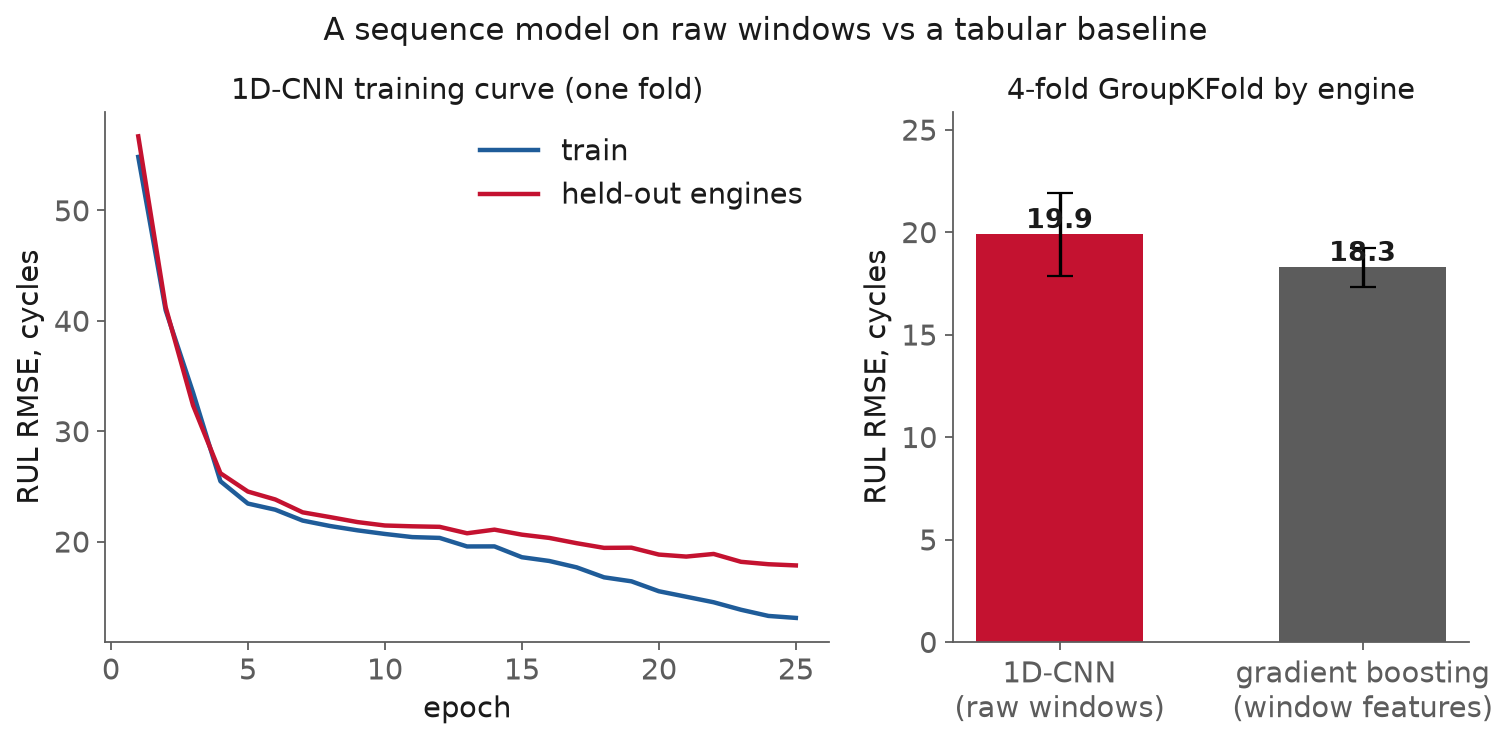
Fig. 74 The 1D-CNN reaches 19.9 plus or minus 2.0 cycles of RUL RMSE across four engine-grouped folds; the tabular baseline on window features reaches 18.3 plus or minus 1.0. The quick sequence model does not beat the strong baseline, and the gap sits inside the CNN’s own fold-to-fold spread.#
The result is the honest one, and it is more useful than a win would be. A convolutional model on the raw signal, the architecture that “should” fit a sensor sequence, lands a cycle or two behind a gradient-boosted tree on simple summary features, and the difference is within the noise. This echoes Lecture 11’s tree-versus-net result and the broader finding of Grinsztajn and colleagues, who benchmarked 45 datasets and concluded that “tree-based models remain state-of-the-art on medium-sized data” of roughly ten thousand samples. The lesson is not that the CNN is bad; it is that a deep architecture earns its advantage from scale, from tuning it properly with the schedule and regularization above, and from data whose structure a hand-crafted feature cannot already capture. On a small, well-summarized benchmark, a strong classical baseline is the model to beat, and beating it is work.
What a practitioner should take from this
Pick the architecture from the shape of the input: an MLP for a vector, a CNN for a field or image, a 1D-CNN or RNN for a sequence, and prefer a temporal CNN to an RNN for fixed windows unless the dependence is genuinely long-range. Fit scalers on training data only and window without crossing unit boundaries, because deep learning does not repeal the leakage rules. Train with a learning-rate schedule and early stopping, and read the loss curves to tell underfitting from overfitting from a bad learning rate. And always run a strong classical baseline: on engineering-scale tabular and windowed data, a deep net is not a default, and a model-family claim from a single run on a leaky split can evaporate when you close the leak and add seeds.
In-class demo#
The notebook trains the lecture’s architectures on C-MAPSS FD001 under one recipe and then asks each of them the questions this session raised. It builds 30-cycle windows over 14 sensors with the piecewise-linear RUL target, and splits by engine: 20 engines are held out for scoring, 12 more decide early stopping, and the rest train, so no engine appears on two sides. A 1D-CNN, a GRU, and a transformer with and without a positional encoding are each trained with the cosine schedule, early stopping, gradient clipping, and weight decay from the training section, with every epoch and the best checkpoint logged to MLflow. Gradient boosting on window summaries and a predict-the-mean floor set the bar on the same scoring engines. The notebook then scores every network on its windows recorded, reversed, and shuffled, and reads the attention weights out of the trained transformer. It is one split rather than the five folds and five seeds behind the tables above, so expect its numbers to differ by a cycle or two and its ordering to hold: boosting in front, the GRU close behind, the transformer without positions scoring the same on all three views, and attention close to uniform. The runnable notebook is l12-cnn-rul.ipynb.
Limitations and trade-offs#
The case for matching the architecture to the input holds, within three limits.
An architecture is an assumption to check#
Choosing a CNN for a field builds in an assumption (locality and translation invariance) that is usually true and occasionally wrong. A global constraint, a boundary condition that couples distant points, or a physical symmetry the plain convolution does not know about, can make the built-in prior a liability. The architecture is a starting hypothesis about the data’s structure, to be checked against a baseline, not a decision that ends the modeling.
Deep networks need more data than engineering datasets often have#
The parameter-sharing economy of a CNN reduces but does not remove deep learning’s appetite for data. A thousand concrete mixes or a hundred engines is small by deep-learning standards, which is precisely why the tree keeps up. When the dataset is small, the honest move is often a strong classical model with good features, and the deep net earns its place as the data grows or as the raw signal carries structure no feature captures.
Accelerators and larger models have costs#
Lecture 11 measured a GPU running a small model 2.5 times slower than the CPU, because the fixed cost of each kernel launch dominates when there is little work to do. More layers, wider layers, and longer training are not free wins either; past the capacity the data can support they buy overfitting and cost time. Match the model size to the data, debug on CPU, and let the accelerator earn its place on a genuinely large run.
Summary#
The one idea of this session is to match the architecture to the structure of the input. A vector goes to an MLP, a field or image to a 2D-CNN, and a sensor sequence to a 1D-CNN or a recurrent network, because a convolution’s parameter sharing and a recurrent state’s memory build in assumptions that are true of that data and would otherwise have to be learned from scratch. For fixed sensor windows a temporal CNN is the sensible default over an RNN, faster to train and often as accurate. Training any of them well means a learning-rate schedule, early stopping on validation loss, gradient clipping, weight decay, and reading the loss curves to separate underfitting from overfitting from a bad optimizer, all tracked in MLflow. The turbofan comparison is the honest anchor: a quick 1D-CNN reaches about 19.9 cycles of RUL error against the baseline’s 18.3, so the sequence model does not automatically win, and a grouped split by engine is what keeps the comparison from lying.
Resources#
PyTorch: Build the Neural Network. Subclassing
nn.Moduleand composing layers, the pattern every model here uses.PyTorch
Conv2dandConv1d. The convolution APIs for fields and for sensor sequences, with thein_channels,out_channels,kernel_size,stride,paddingparameters.PyTorch
LSTM. The recurrent option for long-range sequence dependence.Goodfellow, Bengio, and Courville, Deep Learning, chapters 9 and 10. Convolutional networks and sequence modeling, free online; the sparse-interactions and parameter-sharing argument is chapter 9.
Stanford CS231n: Convolutional Networks. The clearest short treatment of kernels, stride, padding, pooling, and the receptive field.
Bai, Kolter, and Koltun, “An Empirical Evaluation of Generic Convolutional and Recurrent Networks for Sequence Modeling” (arXiv:1803.01271). Why a temporal CNN is a strong default over an RNN.
Grinsztajn, Oyallon, and Varoquaux, “Why do tree-based models still outperform deep learning on typical tabular data?” (NeurIPS 2022, arXiv:2207.08815). The tabular-versus-deep-learning reality check behind the honest baseline.
Smith, “A disciplined approach to neural network hyper-parameters, Part 1” (arXiv:1803.09820). The learning-rate range test and one-cycle schedule, developed in section 4.
Goodfellow, Bengio, and Courville, Deep Learning, chapter 7. Section 7.1.1 derives why weight decay shrinks low-curvature directions most, and section 7.8 shows early stopping acting as L2 regularization and gives the patience algorithm.
Pascanu, Mikolov, and Bengio, “On the difficulty of training Recurrent Neural Networks” (arXiv:1211.5063). Exploding gradients, the steep walls in a recurrent network’s loss surface, and gradient norm clipping (section 3.2, Algorithm 1).
Loshchilov and Hutter, “SGDR: Stochastic Gradient Descent with Warm Restarts” (arXiv:1608.03983). The origin of the cosine annealing schedule that PyTorch’s
CosineAnnealingLRimplements.Loshchilov and Hutter, “Decoupled Weight Decay Regularization” (arXiv:1711.05101). Why
weight_decayin Adam is not true weight decay, and the AdamW fix.NASA C-MAPSS turbofan dataset. Saxena et al. (2008) methodology; the FD001 subset is from the NASA Prognostics data repository, as in Lecture 8.
Assignment#
Assignment 6, “Train a PyTorch model on an engineering dataset,” was released at Lecture 11 and is due about a week later. It asks you to build, train, and honestly evaluate a deep model (an MLP, a CNN, or a sequence model) on a real engineering dataset, using a GPU, with MLflow tracking and a comparison against a strong classical baseline. This session’s architectures and training recipe are what it is built on. This is a pointer, not the rubric.
Practice module#
Practice module for this session, about ten minutes of questions drawn from this session’s notes, slides and demo. It runs entirely in your browser, the questions are selected from your Andrew ID, and it ends by producing a PDF you upload for participation credit.