Lecture 9: The machine learning workflow II, regression

At a glance

• Session Lecture 9, Week 5

• Arc Machine learning and deep learning

• Slides Deck for this session

• Practice Practice module for this session

• Worked example l09-regression.ipynb, to run after class: four model families on concrete strength, and NARX forecasts of reactor pressure

• Tools scikit-learn for the models, the splits and the metrics

Why this matters

Fig. 24 xkcd 1838, “Machine Learning”, by Randall Munroe, CC BY-NC 2.5.

Machine learning (ML) is the field of building models that learn patterns from data. In our case (engineering), instead of explicitly programming rules of physics/nature, we train algorithms to generalize from examples/experimental data. We use it to make predictions on unseen data, to discover patterns in complex systems, and to aid scientific discovery and engineering applications. And sometimes the models that come from first principles can’t fully describe the process we are studying, because the simplifications made the model a weak representation of reality.

Lecture 8 did this for a time series: the rows were minutes of one plant, and their order in time decided what counted as the future. Most of today’s rows have no order. Each row is one experiment on its own: a concrete mix crushed at one age, water held at one temperature, a surfactant solution at one concentration. A model fitted to such a table is often a surrogate, a cheap function that stands in for an expensive simulation or a destructive test. The same kind of table shows up well outside engineering: a wafer that passes or fails inspection, a diagnosis from a patient’s lab values, the price of a house from its size and location.

The comic above is the failure this session is about: pour the data in, and stir the pile until the answers look right. Here is what it looks like in practice. Take water sealed in a rigid container, so that its density stays at 1000 kg/m³, and fit a third-degree polynomial in temperature, \(P = a_3 T^3 + a_2 T^2 + a_1 T + a_0\), to 16 of the 21 pressures the NIST (National Institute of Standards and Technology) Chemistry WebBook gives between 0 and 100 °C: the training \(R^2\) is 0.9999975. Ask the same model about 300 °C and it answers 223 MPa. NIST gives 517.7 MPa. Nothing in the score warned us, because the score only measured the model on data like the data it was fitted to.

The second failure is harder to see. On the concrete data, a decision tree beats a straight line given two physics features when the rows are assigned to folds at random, and loses to it by 2 MPa when the rows are grouped by concrete mix. Same data, same models, same code, and the ranking reverses. This session is about getting that ranking right: how to split the data, which model families to try, what their training actually solves, how to score them, and how to tell a model that learned something from a model that memorized its training rows.

Learning objectives

By the end of this session you should be able to:

• Frame an engineering question as regression or classification, and name its samples, features and target.

• Split data into training, validation and test sets, and explain why the test set is used only once.

• Fit and compare linear, decision tree, neural network and Gaussian process models through scikit-learn’s common fit and predict interface, on a table of experiments and on a NARX table.

• Write the training of a linear model, a neural network and a Gaussian process as an optimization problem, and say what each one optimizes.

• Use k-fold and grouped cross-validation, validation curves and learning curves to diagnose underfitting and overfitting and to choose between models.

The examples in this session

Four datasets carry this session, and a synthetic one helps where a mechanism is easier to see on data whose truth is known. Each is introduced here once, so that the sections after it can use it without stopping to explain where it came from.

Water held at constant density

Picture a fixed mass of liquid water sealed in a rigid container with no room to expand. Its density cannot change, so it stays at 1000 kg/m³, and when the water is heated its pressure climbs steeply: from about 0.4 MPa near 0 °C to about 100 MPa, roughly a thousand atmospheres, at 100 °C. The data are that pressure at 21 temperatures from 0 to 100 °C in steps of 5 °C, from the NIST Chemistry WebBook of the National Institute of Standards and Technology, which computes them from the IAPWS-95 reference equation of state for water (Wagner and Pruss, 2002). It has one input and one output, and its curve is smooth but not straight. It is the example for feature engineering, regularization and the first look at a decision tree. Because NIST also gives the pressure far above 100 °C, it is also the example that shows what each family of models does outside the range of its data.

Surfactant viscosity

A surfactant is a molecule with a water-loving head and a water-avoiding tail, the working ingredient of soaps and shampoos. Some surfactants, mixed with the right salt, self-assemble in water into long, flexible wormlike micelles that tangle like polymer chains and make the solution thick and elastic. The system here is the classic one, the surfactant cetylpyridinium chloride with the salt sodium salicylate, from Rehage and Hoffmann (1988). The measured quantity is the zero-shear viscosity, the viscosity of the solution at rest: the plateau its viscosity curve reaches as the shear rate goes to zero. It sets how thick such a fluid is, which is why wormlike micelles are used commercially as viscosity modifiers, as drag-reducing agents, and in enhanced oil recovery (Pathak and Hudson, 2006). The same effect thickens shampoo. Formulators thicken a shampoo with ordinary salt, too much salt makes it runny again, and the plot of viscosity against added salt is called the salt curve (Romanowski, 2011; Yavrukova et al., 2020, author’s copy). The viscosity at rest is the one a user notices: a thin shampoo is perceived as watered down, and the same viscosity is tied to whether pearlescent pigment stays suspended over the shelf life (Rheology Lab). As the salt concentration rises in the paper’s system, the viscosity climbs steeply to a sharp peak and falls again. The climb is the salt screening the charges of the surfactant heads, so that spherical micelles grow into long worms; the fall past the peak is commonly attributed to the worms branching or shortening, and which of the two happens is still debated (Ziserman et al., 2009).

The sixteen points are not from the 1988 paper itself. The course notes that supply them describe them as experimental data gathered by a design of experiments driven by Gaussian process regression, to replicate the paper’s viscosity curve, for a course in the Kitchin group (06-681 course notes), and those notes label the axis salt concentration and give no units for either axis. In the paper the surfactant is held fixed and the salt is varied (Berret, 2004, figure 7, at 100 mmol/L of surfactant). The sixteen points reproduce the shape of that curve, a sharp peak, a dip, a smaller second peak and a fall, on a compressed scale: across them the viscosity climbs by a factor of about 400, where the paper’s own curve spans about five decades. Sixteen points is a small dataset, which is where a Gaussian process is at its best, so this is the example for Gaussian process regression and for how a Gaussian process chooses its length scale.

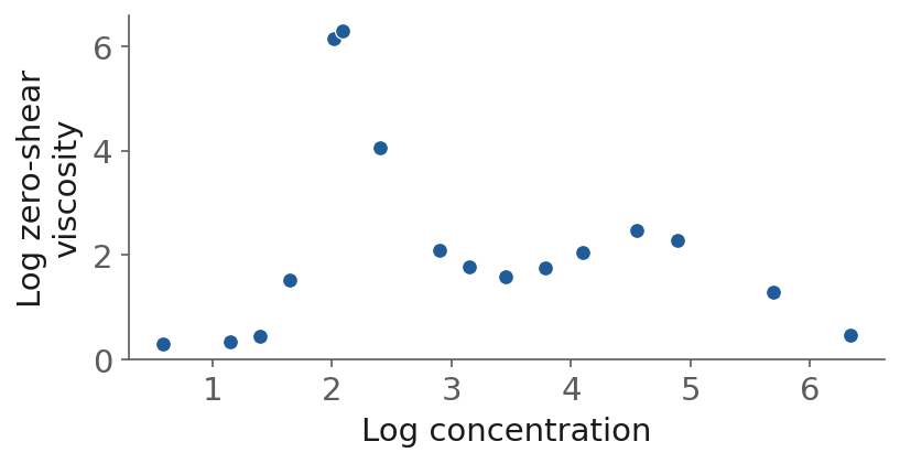
Fig. 25 The sixteen surfactant points, gathered to reproduce the viscosity curve of Rehage and Hoffmann (1988), on (natural) log axes.

Concrete compressive strength

Concrete is cement and water binding sand and gravel (the fine and coarse aggregate) into a rock-like mass (NRMCA). It is the most used material in civil engineering, and the number that decides whether a mix is good enough is its compressive strength: the stress, in MPa, at which a cured concrete cylinder crushes in a testing machine (the test is ASTM C39). Design codes specify it at an age of 28 days (NRMCA), because concrete keeps gaining strength as it cures. One sample is one concrete mix tested at one age. A mix is a recipe: the kilograms of each ingredient in one cubic meter of concrete. The eight features are the amounts of seven ingredients in kg per cubic meter (cement, blast-furnace slag, fly ash, water, superplasticizer, coarse aggregate and fine aggregate) and the age in days. The target is the compressive strength in MPa, which is measured by crushing cylinders cast from the mix, so a model that predicts it from the recipe saves casting cylinders and waiting up to a year to crush them. The data is from Yeh (1998), a set of laboratory trial batches of high-performance concrete (concrete meeting performance and uniformity requirements that ordinary ingredients and practice cannot always reach, in the ACI’s definition) to which Yeh fitted neural networks, and it is on the UCI Machine Learning Repository under CC BY 4.0: 1,030 rows, at ages from 1 to 365 days, with strengths from 2.3 to 82.6 MPa.

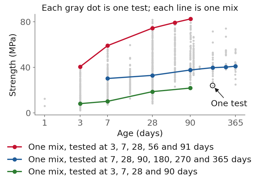
Fig. 26 The concrete data from Yeh (1998). Each gray dot is one test, one mix crushed at one age, and one of them is circled; each colored line follows one mix whose cylinders were crushed at several ages, which matters for the section on cross-validation.

The 1,030 rows are not 1,030 independent experiments. They are 428 distinct mixes, because 182 of the mixes were crushed at several ages, and the section on cross-validation shows how much that changes the answer. Concrete is the main regression example of the session: all four model families are compared on it, and it carries the diagnostics of model capacity.

The Tennessee Eastman process

The simulated chemical plant of Lecture 5 and Lecture 8 (Downs and Vogel, 1993), in the two data files from Rieth et al. (2017): fault-free runs, and faulty runs for faults 1 to 20, with 52 channels (41 measurements and 11 valve positions) sampled every three minutes. Its rows are three-minute samples of a plant, so, unlike the other three datasets, their order matters and they are split by run, as in Lecture 8. Today it supplies Lecture 8’s forecasting table, fitted this time with a network and a Gaussian process.

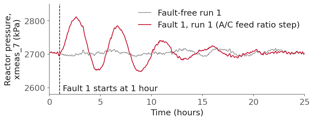
Fig. 27 Reactor pressure in a fault-free run and in a run of fault 1 (a step in the A/C feed ratio), from the training files. The fault starts one hour in, as it does in every faulty training run of Rieth et al. (2017).

A synthetic dataset

The synthetic dataset is \(y = x^{1/3}\) plus Gaussian noise: 120 points on \([0, 1]\) with a noise standard deviation of 0.03. It is where the neural network is built by hand, and the regularization slider in the deck uses 15 noisier points of the same function. On synthetic data the truth is known, which is why it is used to show a mechanism rather than to make a claim about engineering data. One one-off toy appears in the section on neural networks: two inputs on very different scales.

Types of machine learning

Machine learning splits into three types, by what the data comes with.

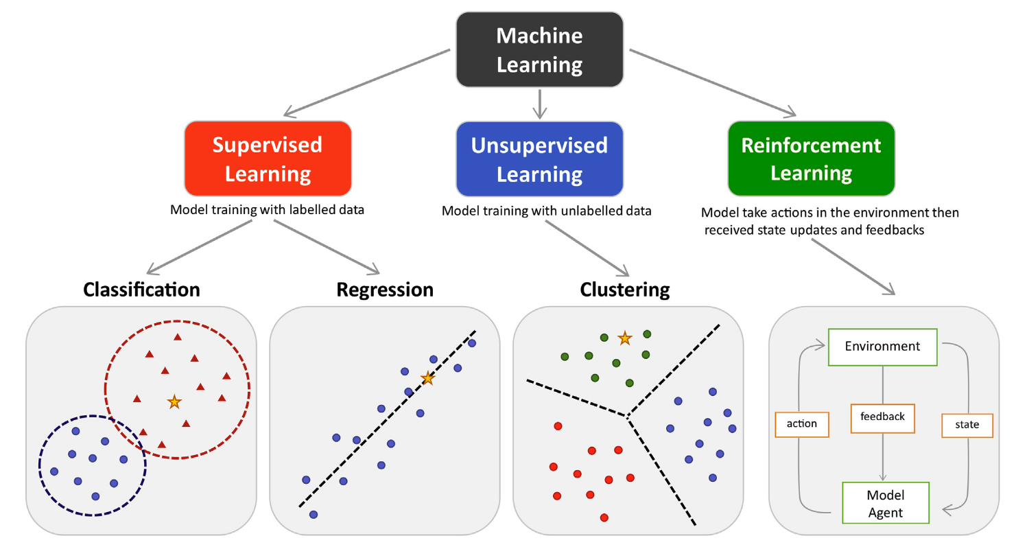
Fig. 28 The three classes/types of machine learning. From Peng, Jury, Dönnes and Ciurtin (2021), Frontiers in Pharmacology 12:720694, CC BY 4.0.

Supervised learning, which Lecture 8 defined, works on data that comes with labels (target outputs). Predicting new values of measurements from previous sensor data and inputs in a chemical plant is supervised learning, and so is everything else in this session. Unsupervised learning works on data that has no labels. The goal is to find hidden structure, and the examples are clustering and dimensionality reduction. Reinforcement learning is the third type: the model takes actions in an environment, receives state updates and feedback, and learns which actions pay off.

Within supervised learning there are two kinds of task, set by the type of the target.

Definition: classification and regression

Classification predicts discrete categories (yes/no, faulty/not faulty, category A/category B, etc.). Regression predicts continuous values (temperature, pressure, flow rates, etc.).

Most of the problems in engineering will fall into the supervised learning/regression category. However, in process control, applications of reinforcement learning and classification (fault diagnosis, for example) are also common. Detecting faults in a plant when nobody has labeled any faults is the unsupervised case.

Some terminology

ML is a bit jargonized. Let’s clarify most of the terms used before we move on:

• Sample (observation, instance, row): a single data point in the dataset. Example: one measurement of water at 50 °C and its pressure.

• Feature (input, independent variable, \(X\)): the input variables used by the model. Example: temperature (water); the seven ingredient amounts and the age (concrete).

• Target (output, label, dependent variable, \(y\)): the value the model is trying to predict. Example: pressure (regression) or phase A against phase B (classification).

• Model: the mathematical function or algorithm that maps features to the target. Examples: linear regression, decision tree.

• Training set: the subset of data used to fit the model parameters.

• Test set: the subset of data held back to evaluate how well the trained model generalizes.

• Prediction (\(\hat{y}\)): the model’s estimated value for the target, given new features.

• Error (residual): the difference between the actual target and the predicted value, \(y - \hat{y}\).

The examples in this vocabulary

Here are the session’s examples again, each one named in these terms.

Example	One sample	Features	Target	Task
Water	One temperature	Temperature (°C)	Pressure (MPa)	Regression
Surfactant	One solution	Log concentration	Log zero-shear viscosity	Regression
Concrete	One mix crushed at one age	Seven ingredients (kg/m³) and the age (days)	Compressive strength (MPa)	Regression
Tennessee Eastman, forecasting	One time step of one run	Ten past reactor pressures and the 11 valve positions now	Reactor pressure 30 minutes later (kPa)	Regression (NARX)
\(y = x^{1/3}\) plus noise	One point	\(x\)	\(y\)	Regression

What changes from Lecture 8

In Lecture 8 a row’s position in time decided everything. The target sat \(h\) rows in the future, and a shuffled split let the model read it. On water and surfactant the rows are separate experiments, the order they sit in the file means nothing, and shuffling them before splitting is allowed. The concrete rows have no time order either, but they are not all separate experiments. The Tennessee Eastman rows are still minutes of a plant, and they are still split by run. There is one catch, and the section on cross-validation comes back to it: separate rows are not always separate experiments, as the 428 concrete mixes showed.

The machine learning workflow

Fitting the model is one step of a structured workflow:

1. Feature engineering. Select or transform the input variables (\(X\)). Examples: using polynomial features of temperature, or building the lagged columns of a NARX table, the regressors of Lecture 7. A transform that is fitted to data, such as scaling, is fitted on the training rows only, after the split.

2. Data splitting. The training set is used to fit the model. The test set is used to evaluate its performance on unseen data.

3. Model selection. Choose appropriate ML algorithms (linear models, trees, etc.).

4. Model validation. Prevent overfitting, using metrics such as \(R^2\) and the mean squared error.

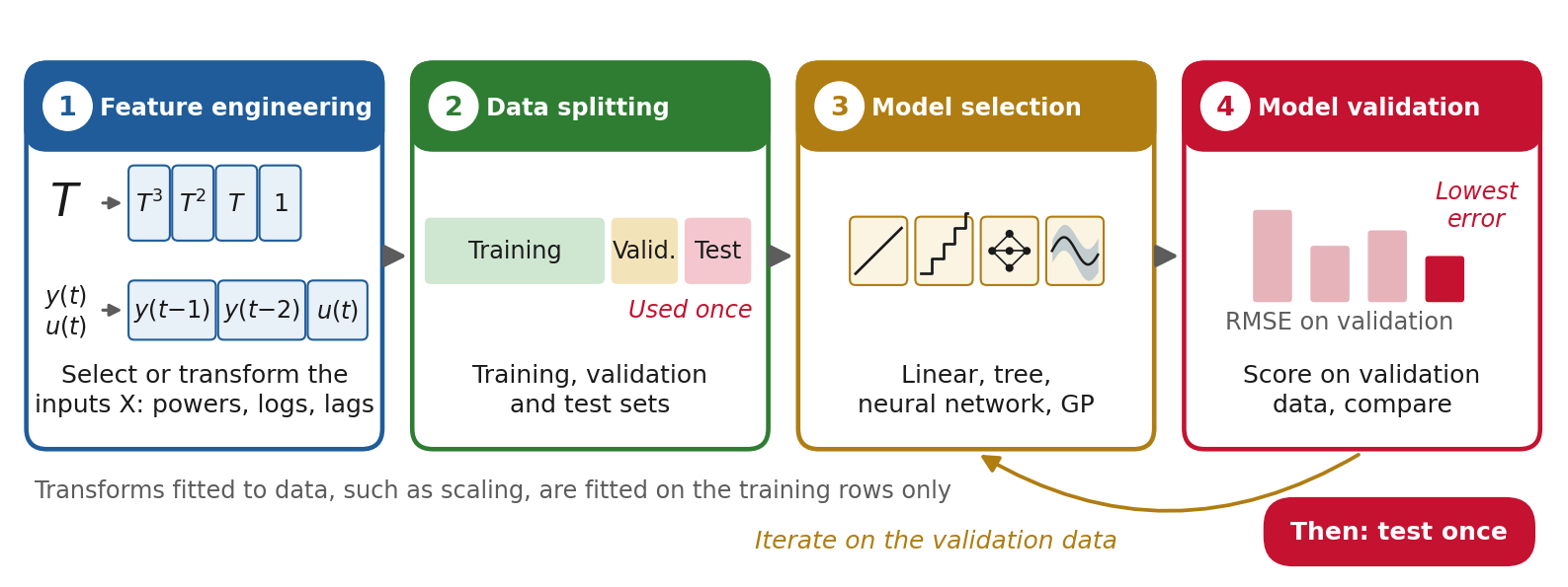
Fig. 29 The four steps. Steps 3 and 4 repeat on the validation data; the test set is used once, at the end.

scikit-learn has a function for step 2:

from sklearn.model_selection import train_test_split

X_train, X_test, y_train, y_test = train_test_split(
    X, y,
    test_size=0.2,
    random_state=42,
)

Two types of validation can be performed: hold-out and cross-validation. Hold-out validation is the most popular one. You hold a percentage of the original dataset for validation/testing purposes. Cross-validation is often used for a more robust evaluation, and it has its own section below.

Training, validation and test sets

Lecture 8 introduced the held-out score, the error on rows the model did not see while fitting. Once you compare several models, one held-out set is not enough, because choosing between models is itself a kind of fitting. So the held-out rows are split once more.

Definition: training, validation and test sets

The training set is used to fit each model’s parameters. The validation set is used to compare models and to choose their hyperparameters. The test set is used once, at the end, to score the one model you chose.

The test set is touched once. Each time you look at a score and change something (a hyperparameter, a feature, the model family, or even the decision to keep trying), information from those rows flows into your choices, and the score stops being an estimate for new data. Validation data is meant to be used that way. Test data is not, and once you have looked at a test score and changed something because of it, the test set has become validation data. The number the test set gives you is the number you report, even when you do not like it.

On the concrete data we lock the test set first: 20% of the mixes (86 mixes, 195 rows), drawn at random and set aside before anything is fitted. Everything else in this session uses the other 835 rows.

Scoring a regression model

Evaluation metrics tell us how well a model is performing. Choosing the right one depends on the type of task (regression or classification) and the goal (the size of a typical error, the cost of a large one, interpretability).

\(R^2\), the coefficient of determination, measures the proportion of the variance in the target explained by the model. It ranges from \(-\infty\) to 1: 1 is a perfect fit, and 0 is what predicting the mean scores.

\[ R^2 = 1 - \frac{\sum (y_i - \hat{y}_i)^2}{\sum (y_i - \bar{y})^2} \]

MSE, the mean squared error, is the average of the squared differences between the actual and the predicted values:

\[ \text{MSE} = \frac{1}{n} \sum (y_i - \hat{y}_i)^2 \]

It penalizes large errors more strongly (by squaring), so it is standard in regression tasks where outliers matter. Its limitation is that its units are squared (°C², MPa²), which are not directly interpretable. RMSE, the root mean squared error, fixes that by taking the square root, \(\text{RMSE} = \sqrt{\text{MSE}}\). It keeps the same heavy penalty on large errors and comes back in the units of the target, so an RMSE of 7 MPa can be compared with a specification.

MAE, the mean absolute error, is the average of the absolute differences:

\[ \text{MAE} = \frac{1}{n} \sum |y_i - \hat{y}_i| \]

It is more interpretable (same units as the target) and less sensitive to outliers than the MSE, but it doesn’t penalize large errors as harshly. The RMSE is never smaller than the MAE, and when it is much larger, a few large errors are hiding among many small ones. For the GP on concrete, under the grouped cross-validation below, the RMSE is 7.17 MPa and the MAE 4.94.

No single number shows where the errors are. A parity plot does: predicted against measured, one point per sample, with the diagonal as the perfect model. Points above the diagonal are over-predictions, and a curve in the cloud is a pattern the model missed. There is one in the section on testing once.

Where is the training here?

When we call .fit in scikit-learn for the linear regression model, it is solving the least squares problem for you, the same problem Lecture 7 solved with numpy.linalg.lstsq. Depending on the model we are training, .fit solves a different optimization problem. We use scikit-learn to train our models because it is one of the most popular ML packages in Python, it has quite an extensive library of ML models, it has really thorough documentation with examples, and it has a consistent syntax among algorithms. Because every model is created, fitted and used the same way, swapping one model for another is a one-line change. The loop below trains four separate models on the same training rows and scores each on the same validation rows, so they can be compared. Nothing is averaged or combined, so each score belongs to one model; combining models into one prediction is a different technique, called an ensemble.

from sklearn.linear_model import LinearRegression
from sklearn.tree import DecisionTreeRegressor
from sklearn.neural_network import MLPRegressor
from sklearn.gaussian_process import GaussianProcessRegressor

models = {
    "linear": LinearRegression(),
    "tree": DecisionTreeRegressor(),
    "neural network": MLPRegressor(),
    "Gaussian process": GaussianProcessRegressor(),
}
for name, model in models.items():
    model.fit(X_train, y_train)        # each learns its own parameters
    y_pred = model.predict(X_valid)    # all scored on the same rows

Training is an optimization problem

Every .fit in this session solves an optimization problem. Written out, it looks like any other problem in process systems engineering, and seeing it that way takes most of the mystery out of “training”. This section writes the general problem once; each model family in the next section is then a choice of the function being fitted, and each one ends with what its own training solves.

A general optimization problem

Start from the problem an engineer already knows:

\[\begin{split} \begin{aligned} \min_{z} \quad & f(z) \\ \text{s.t.} \quad & h(z) = 0 \\ & g(z) \le 0 \end{aligned} \end{split}\]

The decision variables \(z\) are flows, temperatures or a design; the objective \(f\) is a cost, an energy use or a lost yield; the equality constraints \(h\) are the mass and energy balances and equilibrium relations, and the inequality constraints \(g\) are the bounds, purity specifications and safety limits. Choosing the operating point of a reactor to minimize cost, subject to its balances and a temperature limit, has this form.

A model is a function with parameters

A regression model is a function \(\hat{y} = f(x; \theta)\): the inputs \(x\) are the features, the output \(\hat{y}\) is the prediction, and the parameters \(\theta\) set its shape. Training chooses \(\theta\):

\[ \begin{aligned} \min_{\theta} \quad & L(\theta) = \sum_{i=1}^{N} \big(y_i - f(x_i;\theta)\big)^2 \end{aligned} \]

Definition: loss function

The loss function is the objective of training: a number that measures how badly the model with parameters \(\theta\) fits the training data. Training minimizes it over \(\theta\).

Compared with the reactor problem, the roles are reversed. The decision variables are the parameters \(\theta\), the data \((x_i, y_i)\) are fixed constants, the objective is the loss (here the sum of squared errors), and there are usually no constraints: the parameters are free (the Gaussian process will add bounds). Once \(\theta\) is fixed, the trained model \(f(x;\theta)\) is a surrogate, and it can go back into an engineering optimization problem as a constraint, with \(x\) as the decision variables again.

How an optimizer moves

Apart from least squares, which has a closed-form solution, these problems are solved by iteration. Almost every method used to train a model is a variant of one update, familiar from any course on nonlinear programming:

\[ \theta_{k+1} = \theta_k - \eta_k\, H_k\, g_k , \]

where \(\theta_k\) is the current point and \(g_k = \nabla L(\theta_k)\) is the gradient of the loss there. The gradient points uphill, which is why the update subtracts it, and it is computed either from all the rows or from a random mini-batch of a few rows. \(H_k\) is a matrix that rescales the step using the curvature of the loss, and \(H_k = I\), the identity (no rescaling), is plain gradient descent. \(\eta_k\) is the step length, how far to move. The methods differ in two choices: which rows the gradient is computed from, and what \(H_k\) is.

Method	Gradient \(g_k\) from	Step shaping \(H_k\)	Where you meet it
Gradient descent	All the rows	The identity	Textbooks; rarely used as it is
Stochastic gradient descent (SGD)	A small random mini-batch of rows	The identity	Deep learning on large data
Adam	A mini-batch, averaged over steps (momentum)	Diagonal: one step size per parameter, from the running average of \(g^2\)	The default solver of MLPRegressor, and of most deep learning
L-BFGS	All the rows	An estimate of the inverse Hessian built from the last few steps, with a line search	MLPRegressor(solver="lbfgs"), and every Gaussian process fit in scikit-learn

L-BFGS is the quasi-Newton method a process systems engineer already knows from NLP solvers. BFGS builds an approximation of the inverse Hessian from how the gradient changed between iterations, and the limited-memory version keeps only the last few pairs of steps and gradient changes instead of a full matrix, so it scales to many parameters (Liu and Nocedal, 1989). On a smooth problem, with a line search, it needs far fewer iterations than gradient descent. Its cost is that every iteration needs the gradient over all the rows, and its curvature estimate assumes that gradient is exact. So it is the method of choice for small and medium datasets, where a full gradient is cheap, and it is what the MLPRegressor version of the three-unit network, the concrete network and every Gaussian process in this session are trained with. (The minimize fit of the three units uses scipy’s default for an unconstrained problem, full BFGS.)

Stochastic gradient descent gives up the full gradient. Each step uses the gradient of the loss on a small random mini-batch of rows, which is a noisy estimate of the full one (Bottou, Curtis and Nocedal, 2018). A step then costs a mini-batch instead of the whole dataset, so on a million rows you can take thousands of cheap, noisy steps in the time one full gradient would take. The noise has a price: the iterates do not settle unless the step length shrinks.

Adam (Kingma and Ba, 2015) is stochastic gradient descent with two running averages. The average of the gradient is momentum, which smooths the noise. The average of the squared gradient gives each parameter its own step size, so a parameter whose gradients are large takes small steps. Both averages start at zero, so the paper corrects them for that bias in the first iterations. Its suggested defaults, which MLPRegressor also uses, are a step of 0.001 and decay rates of 0.9 and 0.999 for the two averages.

The MLPRegressor documentation puts the practical choice in two sentences: “The default solver ‘adam’ works pretty well on relatively large datasets (with thousands of training samples or more) in terms of both training time and validation score. For small datasets, however, ‘lbfgs’ can converge faster and perform better.” A Gaussian process has no such choice to make. Its default optimizer is L-BFGS-B, the version of L-BFGS that handles bounds on the variables, which the section on Gaussian processes explains the need for.

The figure below runs all four on one small problem: a straight line fitted to the water data. The loss is a quadratic bowl, but a long and narrow one, because the intercept and the slope trade off against each other. Gradient descent takes 305 iterations. L-BFGS learns the shape of the valley from its first few steps and finishes in 6. Stochastic gradient descent, with four rows per step and a fixed step length, reaches the valley floor quickly and then keeps bouncing, because every mini-batch points in a slightly different direction. Adam, run here on the full gradient, overshoots on its momentum and settles in 249.

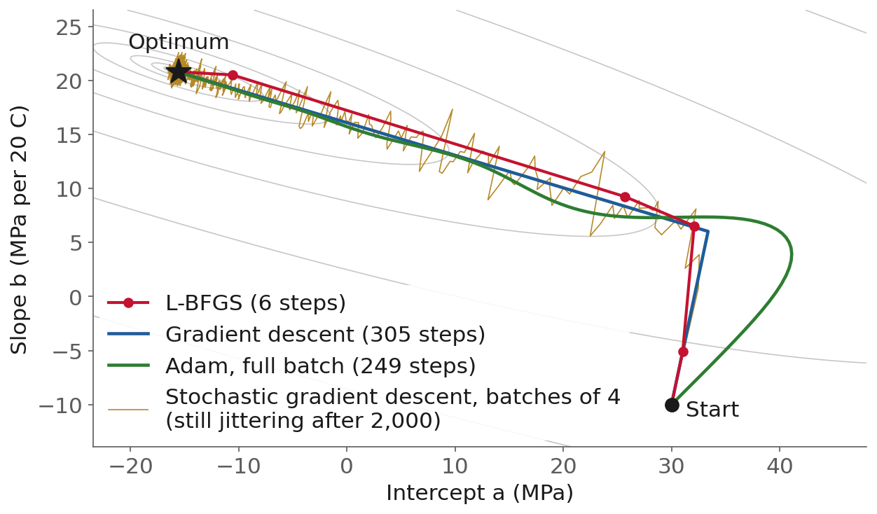
Fig. 30 Four optimizers fitting a straight line to the water data, \(P = a + b\,(T/20)\), by least squares, from the same start, drawn over the contours of the loss. The step counts are to a relative loss gap below \(10^{-6}\); stochastic gradient descent, with mini-batches of 4 rows and a fixed step, never settles. Adam is run here on the full gradient, so it differs from gradient descent only in its update.

Where do the gradients come from? For a network, from backpropagation: the chain rule applied layer by layer, from the loss back to the first weights, which is reverse-mode automatic differentiation (Baydin et al., 2018). For a Gaussian process, scikit-learn differentiates the log marginal likelihood analytically.

Regression models

The four model families below are the ones you will most likely reach on a table of engineering data. Each is shown first on a small example with one input, where you can see what it does, and each ends with what its training solves. Then the linear model, the network and the GP are measured on Lecture 8’s plant table, and all four on concrete, at the end of the section.

Linear regression and feature engineering

The linear regression model has the form

\[ y = \sum_i a_i x_i \]

and the task is to “learn” the coefficients \(a_i\) such that we have a model that explains, as well as possible, the relationship between the inputs and the output. Take the water data from the examples above: pressure against temperature at a density of 1000 kg/m³, 21 points from 0 to 100 °C. The curve is not a straight line, so we give the model more to work with:

X = np.array([T**3, T**2, T, T**0]).T    # columns: T³, T², T, 1

With these columns the model is \(P = a_3 T^3 + a_2 T^2 + a_1 T + a_0\), a third-degree polynomial in temperature.

This is called feature engineering: transforming raw inputs into a form that makes the relationship easier for the model to capture. We got our raw temperature measurements, we looked at the data, and we created a feature vector \(X\) that is a realization of \(T^0, T^1, T^2, T^3\). This is very common in ML tasks. The model is still linear in its coefficients, and .fit still solves a least squares problem.

Definition: feature engineering

Feature engineering is transforming raw inputs into a form that makes the relationship easier for the model to capture: powers, logarithms, ratios, or the lagged columns of a NARX table.

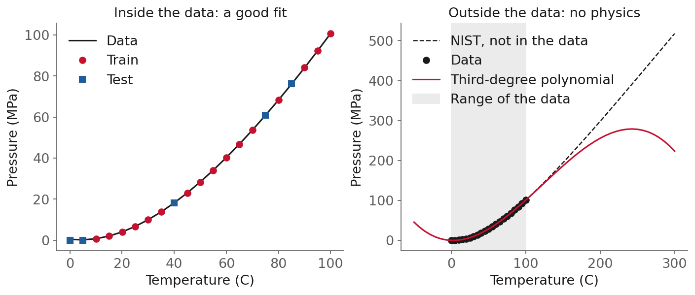
Fig. 31 Left: a third-degree polynomial in temperature, fitted on 16 of the 21 NIST points (red) and checked on the other 5 (blue). Right: the same model from −50 to 300 °C. The dashed line is the NIST isochore beyond the data, which the model never saw.

The fit scores \(R^2 = 0.9999975\) on the training points and 0.99994 on the five test points. Note that this is merely a polynomial model, so you should not use it for extrapolation. Although it was fitted using a library that implies machine learning was employed, there are no physical principles incorporated into this model. It shows incorrect behavior at both low and very high temperatures: at −50 °C it predicts 45.6 MPa, and at 300 °C it predicts 223 MPa, where NIST gives 517.7. Within the data range, it is a reasonable estimation.

On the concrete data the same idea earns more. A linear regression on the eight raw columns scores 10.6 MPa of root mean squared error in five-fold cross-validation, against 16.8 MPa for predicting the mean (the RMSE was defined in the workflow section, and cross-validation has a section of its own below). Two features built from what concrete engineers already know, bring it to 7.25 MPa. The first is the logarithm of the age, because concrete gains strength fast in its first days and slowly after: the mean strength in this file is 19.0 MPa at 3 days, 26.1 at 7, 36.7 at 28, 40.5 at 90 and 43.6 at 365. The second is the water-to-cement ratio. Abrams (1918) plotted the compressive strength of many mixes against their water ratio, found one smooth curve, and fitted it as \(S = A/B^x\), where \(x\) is the volume of water per volume of cement. The dataset gives the ratio by mass, which differs from Abrams’s by a constant factor.

Regularization: ridge and lasso

So far we fit models by minimizing the sum of squared errors between the predictions and the data. Two questions remain: which inputs (features) should we be using, and how do we eliminate unnecessary or unhelpful inputs? When we choose by hand which columns go into the model, that is feature engineering. Sometimes we don’t know in advance which features are useful. One approach is to create a library of candidate features (polynomial expansions, for example) and then let the model decide which ones matter. This is where regularization comes in: add a penalty on the coefficients to the training problem,

\[ \min_{a} \;\; \sum_{i} \big(y_i - \hat{y}_i\big)^2 \; + \; \alpha \sum_{j} a_j^2 . \]

Definition: regularization

Regularization adds a penalty on the model coefficients to the loss function, as in \(\text{Loss} = \sum (y_{\text{pred}} - y_{\text{true}})^2 + \alpha \sum a_i^2\). The first term is the usual squared error (the fit to the data). The second penalizes large coefficients, and \(\alpha\) controls its strength.

A large \(\alpha\) gives heavy shrinkage, a simpler model and a risk of underfitting. A small \(\alpha\) keeps the model close to plain linear regression. The penalty above, on the squares of the coefficients, is ridge regression (an L2 penalty), which Lecture 8 used to steady nearly identical lag columns. It shrinks the coefficients of inputs that contribute little, but rarely to exactly zero. Lasso regression (an L1 penalty) adds the absolute values of the coefficients instead,

\[ \text{Loss} = \sum (y_{\text{pred}} - y_{\text{true}})^2 + \alpha \sum |a_i|, \]

which encourages sparsity: lasso sets the coefficient of an input to exactly zero when it is not contributing to the behavior of the output, so some features are removed automatically. Its advantage is this feature selection, which helps interpretability. The trade-off is that the choice of \(\alpha\) is crucial: too large and the model underfits, too small and you get no benefit.

Let’s see how \(\alpha\) affects the parameters on the water data. It is useful to search across a broad range of values, so we use a logspace from \(\alpha = 10^{-15}\) to \(10^4\):

for a in np.logspace(-15, 4, 10):
    model = linear_model.Lasso(
        alpha=a,
        max_iter=50000,
    )
    model.fit(X_train, y_train)

\(\alpha\)	\(T^3\)	\(T^2\)	\(T\)	Training \(R^2\)
\(10^{-15}\)	\(-3.96\times10^{-5}\)	0.01469	−0.0661	0.9999974
\(4.6\times10^{-3}\)	\(-3.94\times10^{-5}\)	0.01467	−0.0649	0.9999973
0.60	\(-3.13\times10^{-5}\)	0.01330	0	0.9999785
77	\(-2.89\times10^{-5}\)	0.01305	0	0.9999565
\(10^4\)	\(9.97\times10^{-5}\)	0	0	0.9559622

With some regularization, the linear term is removed and the fit barely changes. (Even the first row is not exactly least squares: on these unscaled columns, where \(T^3\) reaches \(10^6\), the coordinate descent stops on its tolerance a little short of the least squares coefficients, which is one more reason for the scaling caution below.) With a lot, only one term survives and the fit gets visibly worse. (The coefficient on \(T^0\) is always zero because the model’s intercept absorbs it.)

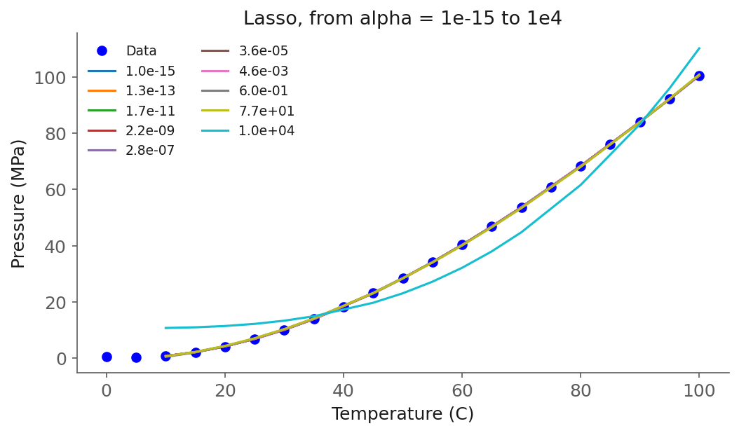
Fig. 32 The lasso fits for ten values of \(\alpha\). Nine of them lie on top of each other; only \(\alpha = 10^4\), which keeps only \(T^3\), visibly departs from the data.

The deck’s live slider makes the trade-off visible on a harder case: 15 noisy points of \(y = x^{1/3}\) fitted with a 12th-degree polynomial, so 12 candidate features, and scored on 80 new points. With \(\alpha\) near zero the curve chases the noise, so the training error is low and the test error is higher. As \(\alpha\) grows the curve smooths and the test error falls; past a point both errors rise, because the model is now too simple. Switched to lasso, the count of nonzero coefficients falls as \(\alpha\) grows. The slider’s right panel, error against \(\alpha\), is a validation curve, the tool of the section on model capacity.

One caution that the water example hides: the penalty treats every coefficient the same way, so the columns have to be on comparable scales before it means anything. Here \(T^3\) reaches \(10^6\) while \(T\) stops at 100. Lecture 8 made the same point for ridge, and put a StandardScaler inside a Pipeline to handle it.

What its training solves. The \(\alpha\) term added to the training problem is a penalty in the sense of penalty methods. Instead of a hard constraint, it adds the size of the coefficients to the objective with a weight \(\alpha\). The lasso is the same idea with absolute values, and in neural networks the squared penalty is called weight decay; it is the alpha of MLPRegressor. Ridge stays a convex quadratic, solved in one linear solve. The lasso’s absolute values keep the problem convex but not smooth, which is why scikit-learn solves it iteratively. And the penalty need not be on the coefficients. It can be the residual of a law the model must obey, a mass balance or a differential equation evaluated at chosen points, \(\lambda \sum_j \lVert \mathcal{F}[f](z_j) \rVert^2\), added to the same training problem; that is the idea behind physics-informed training (Raissi, Perdikaris and Karniadakis, 2019). We will see this later in this course.

Four model families, and why more than one

A linear model bends only the way its features let it, and someone has to choose those features. The three model families after it learn the shape from the data, each in a different way: a tree cuts the input space into boxes, a neural network builds its own nonlinear features, and a Gaussian process puts a probability distribution over functions. Why learn four instead of the best one? Because there is no best one. The no free lunch theorem for supervised learning makes that precise. Loosely speaking, for any two learning algorithms there are “as many” problems on which the first has the lower error on data outside the training set as problems on which the second does (Wolpert, 1996). “As many” is shorthand for an average: weight every possible input-output relationship equally, and every algorithm’s expected error on inputs outside the training set comes out the same. The surprise is in the next sentence of the abstract: this holds even when one algorithm is cross-validation and the other is “anti-cross-validation”, which picks the model with the largest validation error. Averaged over every conceivable problem, nothing wins. More details on the paper (Wolpert, 1996).

A certain type of ML model wins when its assumptions (smoothness for a Gaussian process, boxes for a tree, the right features for a line) match the problem in front of you. So in practice the model is a choice made for each problem, by validation. That step goes beyond the theorem, since trusting validation rests on an implicit assumption about which problems arise, one Wolpert calls difficult to express mathematically and notes that nobody debates (Wolpert, 2020). This session’s own results show the ranking move. On concrete the tree beats the linear model with physics features under one way of splitting the data and loses to it under another, and on Lecture 8’s plant table a network and a Gaussian process tie a linear model.

	Linear, with features	Decision tree	Neural network	Gaussian process
The idea	A weighted sum of chosen features	Yes/no questions, one constant per region	Layers of weights, biases and activations	A distribution over functions, set by a kernel
Good at	Little data; known physics in the features; readable coefficients	Nonlinear, interacting inputs; no scaling needed; readable rules	Any smooth nonlinear shape; many inputs; large data	Small data; smooth functions; an uncertainty with every prediction
Bad at	Shapes its features cannot express	Smooth functions (a staircase); memorizing groups	Small data; scaling; many hyperparameters; local minima; interpretability	Large \(N\), as \(\mathcal{O}(N^3)\); the choice of kernel; scaling
Outside the data	Follows its features (the polynomial bends over)	Flat at the edge leaf	Saturates	Reverts to the mean, with a wide band

The last row is demonstrated in the section on limitations, on the water data.

Decision trees

Definition: decision tree

A decision tree is a nonlinear model that splits the data into regions with a sequence of yes/no questions on the inputs, and predicts one constant value in each region.

Compared with linear regression, trees can capture nonlinearities better. However, they can overfit if their depth is too large, so hyperparameter tuning (max_depth, for example) is crucial. Here is a tree of depth 2 on the water data:

from sklearn.tree import DecisionTreeRegressor

tree = DecisionTreeRegressor(
    max_depth=2,
    random_state=0,
)
tree.fit(T_train.reshape(-1, 1), P_train)    # temperature alone: a tree needs no T**2 or T**3

It scores \(R^2 = 0.911\) on the test points. Something interesting is happening in the plot: the prediction is a staircase, and the tree drawn next to it shows why, more clearly than the equations would.

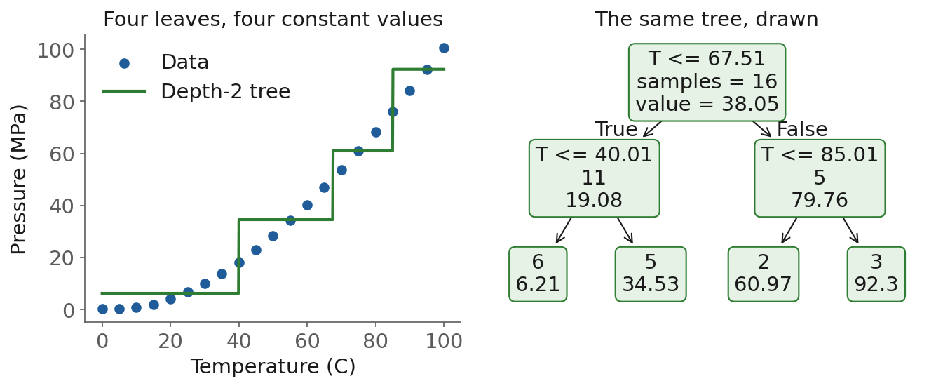
Fig. 33 A depth-2 tree on the water data. Each leaf predicts the average pressure of the training points that reach it.

The decision tree algorithm is dividing/splitting the dataset based on a boundary which gives the minimum MSE. The first question is “is \(T \le 67.5\) °C?”, and each side asks one more question. This is done until every data point is represented by an interval, or until the depth limit stops it. A depth-2 tree has four leaves, so it predicts one of four pressures for any temperature you give it, and its curve is a staircase. A deeper tree has more and smaller steps, and a tree with no depth limit keeps splitting until each leaf holds a single training point.

A tree does not have to predict a constant in each leaf. In Dr. Laird’s group here at CMU we constantly use linear model decision trees, with a linear model in each leaf, as machine learning models for optimization purposes; Ammari et al. (2023) is an example. The linear-tree package builds them on top of scikit-learn, and OMLT translates trained trees and networks into Pyomo optimization models.

What its training solves. A decision tree is not a continuous optimization at all. Finding the best tree is a combinatorial problem, and building an optimal binary decision tree is nontrivial (Hyafil and Rivest, 1976). There is no gradient and no starting point, which is why the solvers of the optimization section do not directly apply to trees.

Neural networks

In engineering we often face nonlinear models (reaction kinetics, transport, thermodynamics), and linear and polynomial regression are limited in flexibility. Neural networks (NNs) emerged in the 1940s and 1950s, inspired by biological neurons, were revived in the 1980s, and became dominant in the 2010s with deep learning applications. Today we use them as universal function approximators. Just as we expanded features with polynomials, NNs expand the feature space adaptively, by learning nonlinear transformations.

Trivia: a Nobel Prize for neural networks

The 2024 Nobel Prize in Physics went to John Hopfield and Geoffrey Hinton, “in recognition of their foundational work in machine learning with artificial neural networks”. Hinton was on the CMU computer science faculty from 1982 to 1987 (CMU News).

A flexible nonlinear regression. We’ll model a noisy nonlinear function. Let the data be defined by this true function:

\[ y = x^{1/3} + \epsilon, \qquad \epsilon \sim \mathcal{N}(0, \sigma^2), \]

and try the following functional form, with three nonlinear units:

\[ f(x;\theta) = b_1 + w_{10}\tanh(w_{00}x+b_{00}) + w_{11}\tanh(w_{01}x+b_{01}) + w_{12}\tanh(w_{02}x+b_{02}). \]

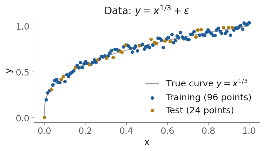
Fig. 34 The data: \(y = x^{1/3}\) plus noise, 96 training and 24 test points.

We fit the ten parameters \(\theta=\{b_1, w_{10}, w_{00}, b_{00}, w_{11}, w_{01}, b_{01}, w_{12}, w_{02}, b_{02}\}\) by curve fitting: minimizing the sum of squared errors with scipy.optimize.minimize, on 80% of 120 noisy points. The fit scores \(R^2 = 0.948\) on the other 20%.

So far, what we have really done is a nonlinear regression, just with an unusual-looking functional form. This model is flexible: it can fit a wide variety of nonlinear shapes, and we could give it a different nonlinear function than tanh and a different number of parameters. But this model did not come out of nowhere. If we allow tanh to act element-wise on a vector, we can write the three-unit model more compactly as

\[\begin{split} y = \begin{bmatrix} w_{10} & w_{11} & w_{12} \end{bmatrix} \tanh\!\left( \begin{bmatrix} w_{00}\,x + b_{00} \\ w_{01}\,x + b_{01} \\ w_{02}\,x + b_{02} \end{bmatrix} \right) + b_1, \end{split}\]

and even more clearly in matrix notation:

\[ y = w^{(1)} \tanh\!\big(W^{(0)} x + b^{(0)}\big) + b^{(1)}. \]

Read it from the inside out. Start with the input \(x\). Multiply by a set of weights \(W^{(0)}\), add a vector of biases \(b^{(0)}\), and apply a nonlinear activation function \(\tanh(\cdot)\). Then multiply by a new set of weights \(w^{(1)}\) and add a final bias \(b^{(1)}\). The result is the output \(y\). This construction is exactly what we call a neural network: an input layer (\(x\)), one hidden layer with three nonlinear units activated by tanh, and an output layer with a linear activation.

Definition: neural network

A neural network is a function built from layers. Each layer multiplies its input by a matrix of weights, adds a vector of biases, and applies a nonlinear activation function. The weights and biases are the parameters that training adjusts.

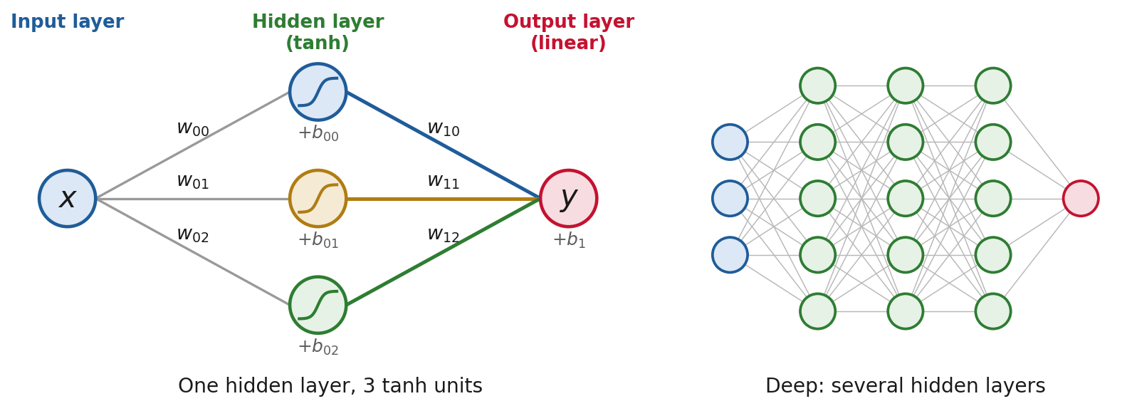
Fig. 35 Left: the three-unit model drawn as a network, one input, one hidden layer of three tanh units and one linear output, with the weights and biases named as in the equations above. Right: a deep network, with several hidden layers.

The figure below shows how the three terms of the equation build the fit. Each hidden unit contributes one tanh-shaped piece, \(w_{1k}\tanh(w_{0k}x + b_{0k})\): here unit 3 makes the steep rise near zero, unit 1 a steady slope, and unit 2 only a small kink at the end. The fitted terms are large numbers that nearly cancel (their offsets are about \(-37\), \(-23\) and \(+64\)), so each is drawn shifted to start at zero; the offsets and the bias \(b_1\) fold into one constant. The output adds the pieces, and the sum is the curve through the data.

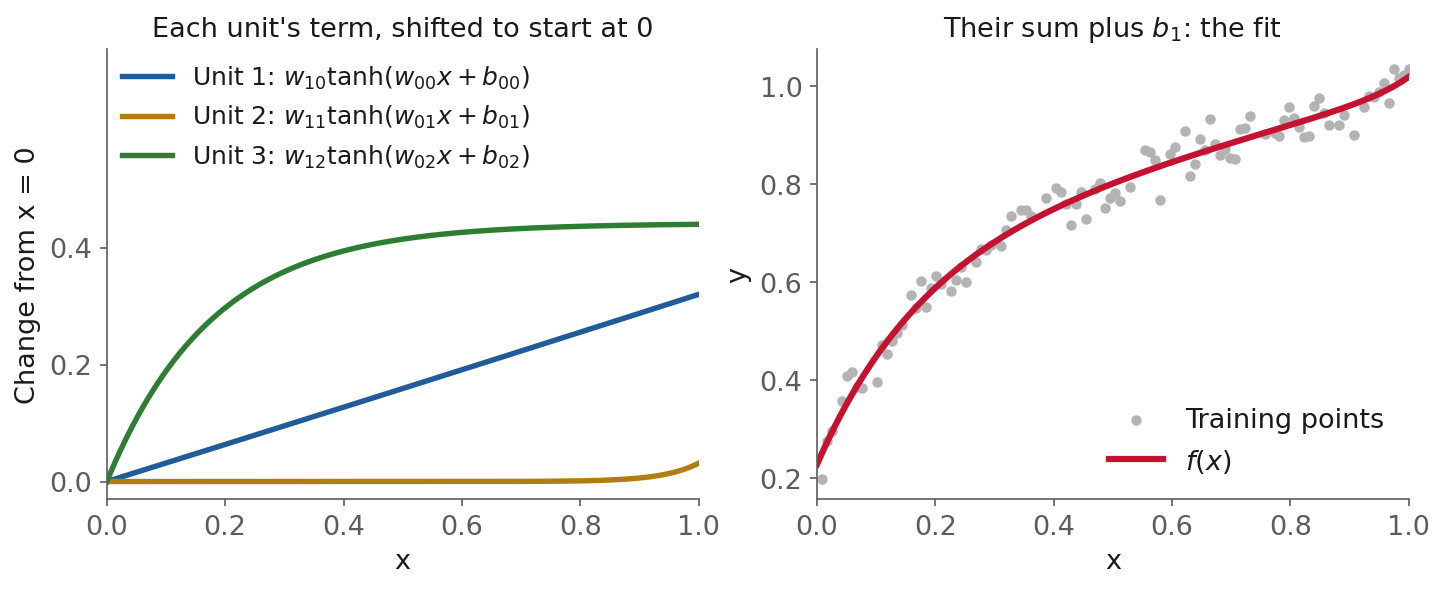
Fig. 36 The three units’ terms, in the colors of the network diagram, and their sum plus \(b_1\), which is the fit.

Stacking more hidden layers, each feeding the next, gives a deep network, which is where the name deep learning comes from. Every layer is the same construction: weights, biases and an activation.

Why “neural” networks? The terminology comes from biology: neurons take signals from inputs, combine them, and if the signal is strong enough they “fire”. The activation function (here, tanh) is a smooth, differentiable approximation of that behavior. Although modern networks are far removed from actual brains, the language stuck. The activation most used today, the rectified linear unit or ReLU, \(\max(0, z)\), is closer to the fire-or-not picture: a unit outputs zero until its weighted input crosses zero, and grows linearly after that. A network of ReLU units is therefore piecewise linear, with a kink wherever one of its units switches on. The deck shows it live with five ReLU units (MLPRegressor, L-BFGS) fitted to the \(y = x^{1/3}\) data: as \(x\) moves, each unit lights up when its weighted input passes zero, and every kink in the fitted curve is one unit switching on or off; one of the five stays on across the whole range and only adds a straight line. A key theoretical result is that neural networks with at least one hidden layer are universal function approximators: in principle, they can represent any continuous function if given enough hidden units.

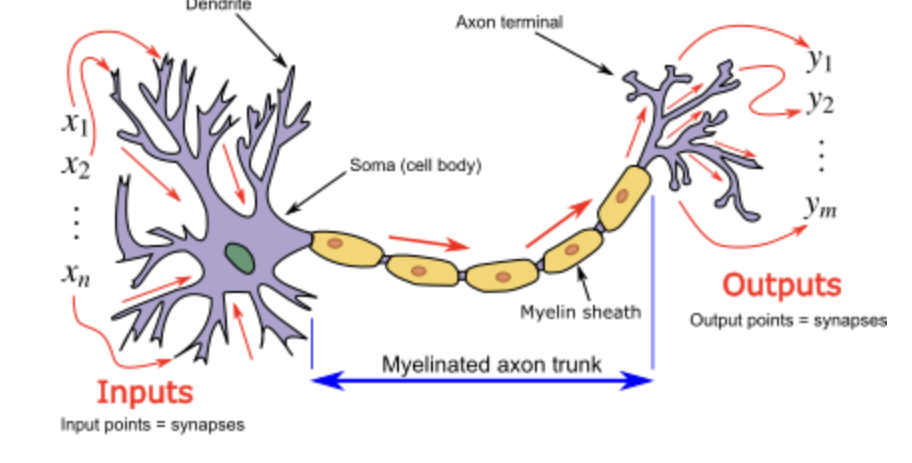
Fig. 37 A biological neuron, with its inputs and outputs labeled the way a network labels them. Neuron3.png by Egm4313.s12 (Prof. Loc Vu-Quoc), Wikimedia Commons, CC BY-SA 3.0.

Design choices are hyperparameters. When we build a neural network, we choose the number of layers (one hidden layer here, and we can stack more to increase flexibility), the number of neurons per layer (more neurons mean more parameters and more capacity to fit complex patterns), and the activation function (tanh and the sigmoid are the classics, and ReLU is the common default today). These are the hyperparameters Lecture 8 defined: they set the model’s size and shape, but they are not themselves fitted during training. Choosing them is often based on experience and experimentation.

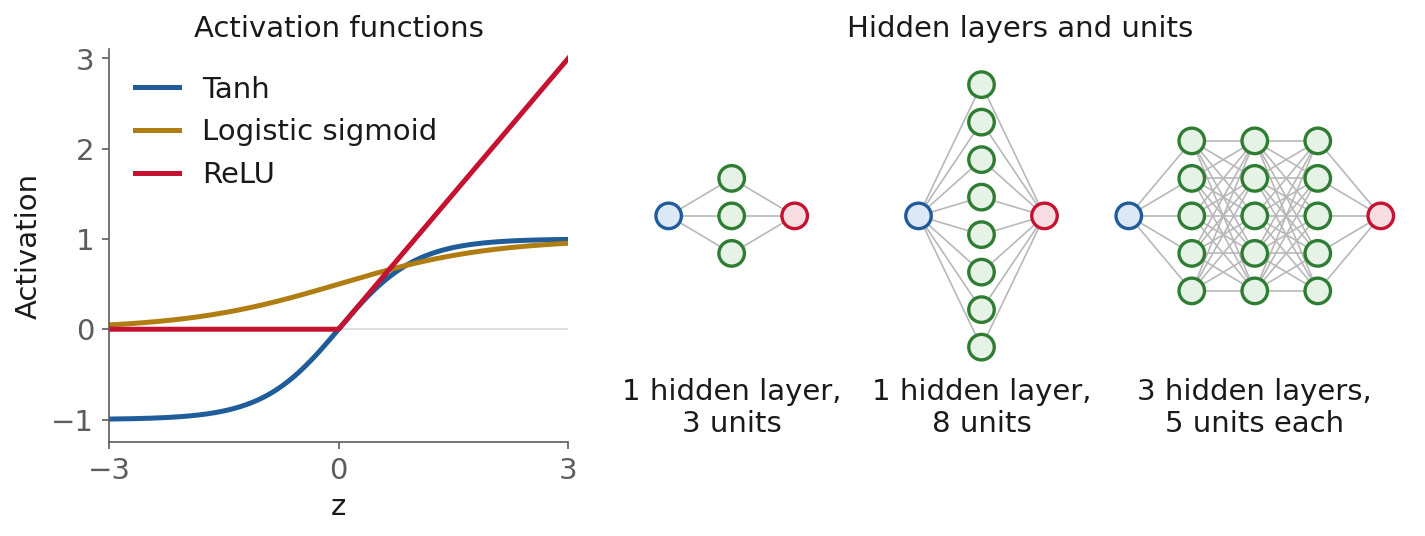
Fig. 38 Three hyperparameters of a network: the activation function, and the number of hidden layers and of units in each.

The same model in scikit-learn. The parameters minimize found above are exactly the weights and biases of a one-hidden-layer network, so scikit-learn’s MLPRegressor (MLP: multi-layer perceptron) fits the same model in one line, and scores \(R^2 = 0.950\) on the same test points. What its .fit solves, and why it can end somewhere different each time, comes right after the code.

from sklearn.neural_network import MLPRegressor

NN = MLPRegressor(
    hidden_layer_sizes=(3,),
    activation="tanh",
    solver="lbfgs",
    alpha=0.0,
    max_iter=5000,
    random_state=0,
)
NN.fit(X_train, y_train)

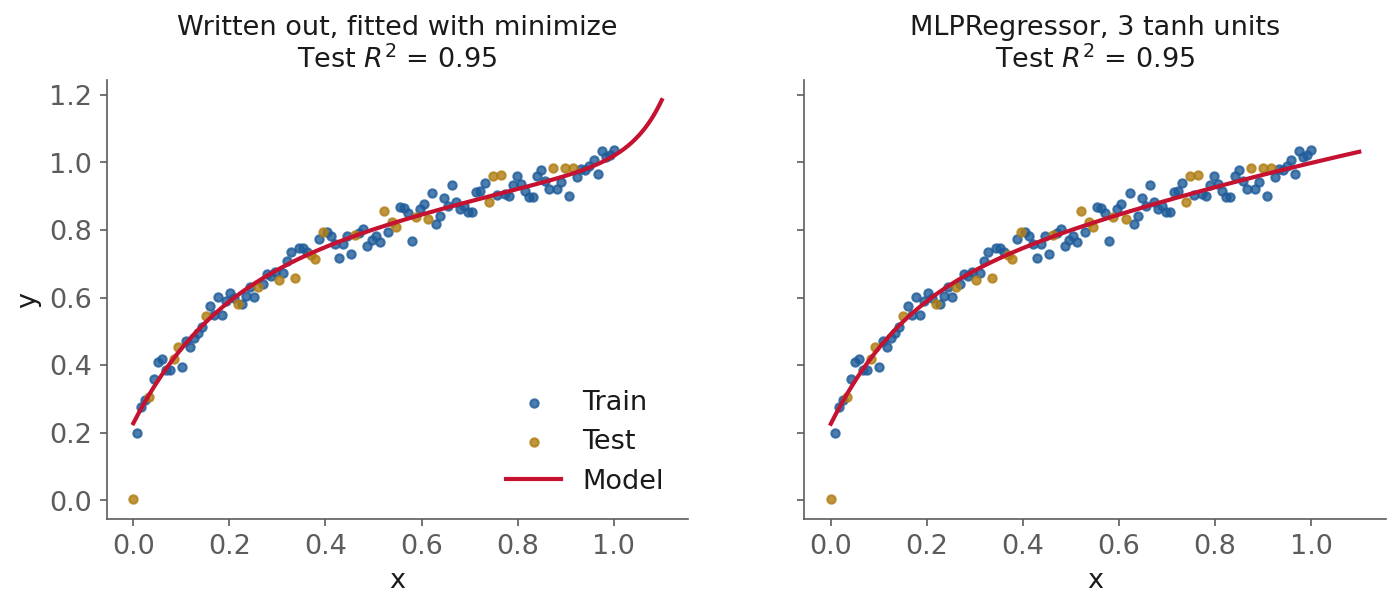
Fig. 39 The same model twice. Left: the three tanh units written out and fitted with scipy.optimize.minimize. Right: MLPRegressor with three tanh units and L-BFGS. Both curves continue past \(x = 1\), where there is no data.

What its training solves. Training a neural network means solving an optimization problem:

\[ \min_{W,b} \sum_{i=1}^N \big(y_i - f(x_i; W, b)\big)^2 \]

The objective is the squared error, and the variables are the network parameters, the weights \(W\) and the biases \(b\). The method is one of the gradient-based methods of the optimization section (L-BFGS here, Adam or stochastic gradient descent on large data), with the gradients computed by backpropagation. The challenge is that the problem is non-convex: it has multiple local minima, and it is sensitive to the initial guess. scikit-learn hides the optimization when we call .fit, but understanding it helps interpret convergence and its warnings. Train the three-unit network from above ten times, changing only random_state, which sets the starting weights:

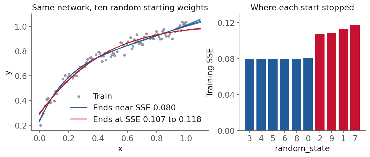
Fig. 40 The same network and the same data, trained from ten random starting weights with L-BFGS. Six starts end near a training SSE of 0.080 (blue); four stop at 0.107 to 0.118 (red).

The final training error ranges from 0.0796 to 0.1177, a factor of 1.48, and the test \(R^2\) from 0.920 to 0.950. Six starts ended within 2% of each other, near 0.080, and four stopped at 0.107 to 0.118. This is why every network in this session is given a random_state: without it, a rerun lands in a different minimum and prints a different number.

Scaling! Consider a dataset with two features on very different scales, \(x_1 \in [0,1]\) and \(x_2 \in [0, 10^6]\), and a target \(y = 0.7\sin(2\pi x_1) + 0.3\,x_2/10^6\). Both features matter for predicting \(y\), but they are on completely different scales. If we train a neural network without scaling, the huge values of \(x_2\) dominate the learning process, and the optimizer struggles to adjust the weights and biases: the network scores \(R^2 = -0.006\) on test data, which is worse than predicting the mean. What happens is precise: with \(x_2\) in the millions, every tanh unit saturates at \(\pm 1\) on every training row, the gradients through a saturated tanh vanish, and the network can only fit a constant, the training mean. If we standardize the features first (zero mean, unit variance), both are on equal footing, and the network learns the relationship: \(R^2 = 0.9999\). Put the scaler inside a Pipeline, as in Lecture 8, so that it is fitted on the training rows only.

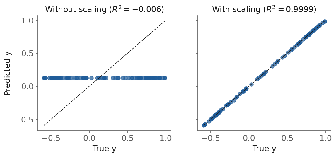
Fig. 41 The same network, trained without and with a StandardScaler. Without scaling it predicts nearly the same value for every sample.

To sum up: a neural network is nonlinear regression with weights, biases and activations. Training adjusts the weights and biases to minimize a loss, and with enough units a network can approximate any (hopefully) continuous function. Its strengths are flexibility and power. Its weaknesses are many parameters, sensitivity to scaling and initialization, and less interpretability. Most important: neural networks are just math, not magic.

Gaussian processes

Neural networks give flexible parametric function fits. Gaussian processes (GPs) take a different route: they put a distribution over functions and deliver predictions with uncertainty. In the parametric view (a neural network, for example), you choose a finite set of parameters \(\theta\) and then fit \(f(x;\theta)\). In the nonparametric view (a GP), you specify a prior over functions, \(f\sim\mathcal{GP}(m,k)\), and conditioning on the data yields a posterior over functions. Instead of committing to one curve, a GP reasons over many plausible curves consistent with the observed data.

Definition: Gaussian process

A Gaussian process is a probability distribution over functions, set by a mean function and a kernel. Precisely: any collection of its function values is jointly Gaussian (normal). To define one we only need a mean function \(m(x)\) (the average shape) and a covariance function, or kernel, \(k(x, x')\) (how similar two points are). We write \(f(x) \sim \mathcal{GP}\big(m(x), k(x,x')\big)\).

The same way one can generalize observed, continuous data as a Gaussian distribution of numbers, one can generalize a function, such as a chemical process model, as a distribution of functions, and that distribution is a Gaussian process.

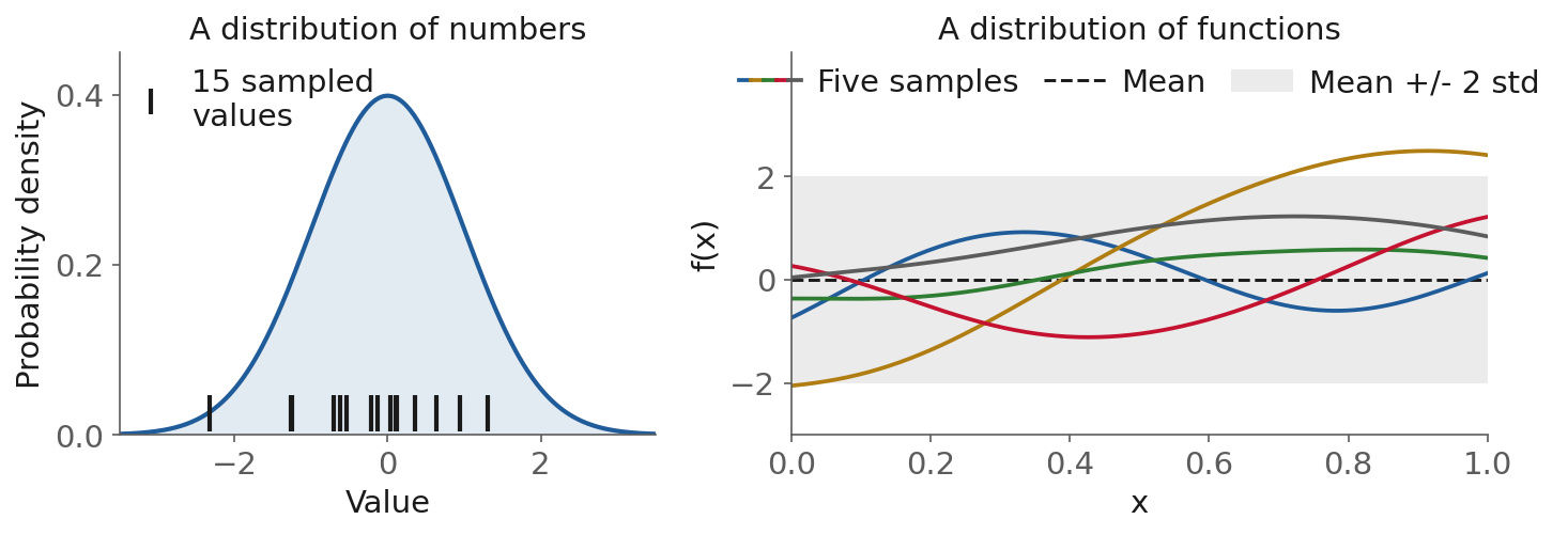
Fig. 42 A distribution of numbers (left) and a distribution of functions (right): five functions drawn from a Gaussian process prior with an RBF kernel.

Learning from data is Bayesian inference. The prior says which functions are plausible before any data; the data then reweight them:

\[ \text{posterior} = \frac{\text{likelihood} \times \text{prior}}{\text{marginal likelihood}}. \]

The posterior is again a Gaussian process, and each new observation pulls its mean toward the data and shrinks its uncertainty near that point, while far from the data the uncertainty stays wide.

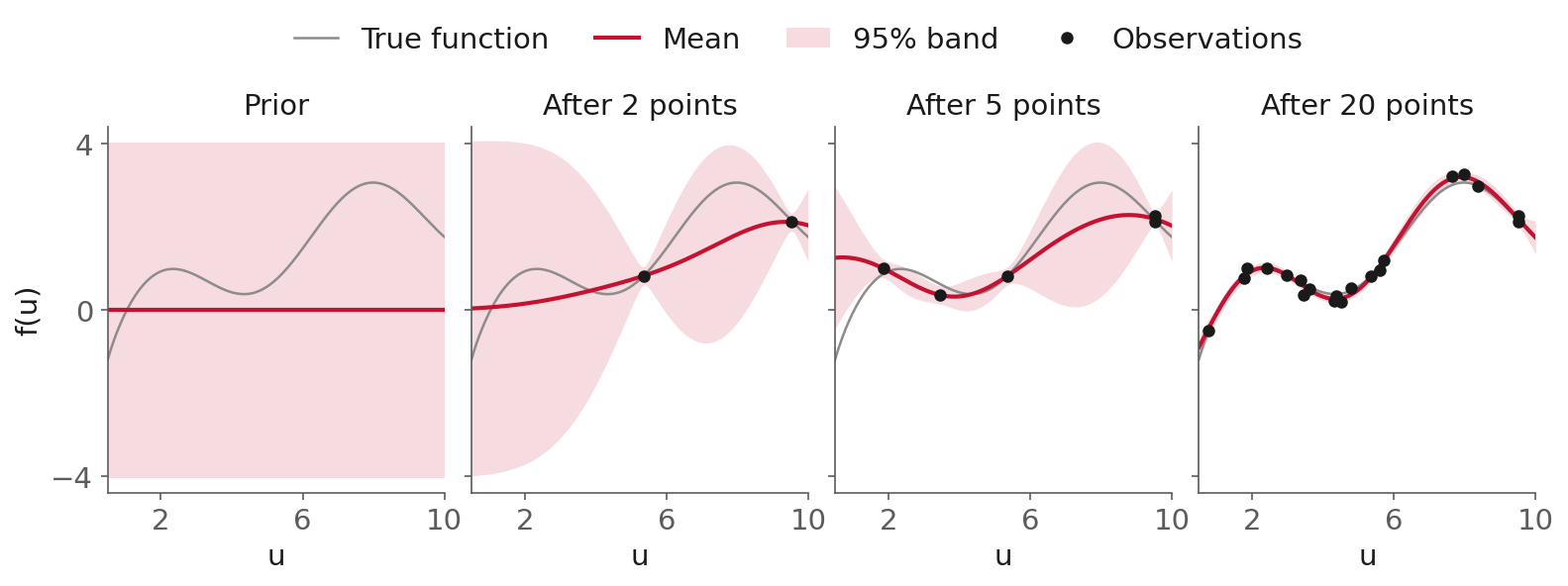
Fig. 43 A Gaussian process learning \(f(u) = \sin u + \log u - e^{-0.1u^2}\), from the prior to the posterior after 2, 5 and 20 noisy observations. The kernel is held fixed, so only the data change.

Suppose we have training data \((x_i, y_i)\) with some Gaussian noise. For a new point \(x_*\), the predicted mean (best guess) and the predicted variance (uncertainty) are

\[ \mu(x_*) = \mathbf{k}_*^\top (K + \sigma_n^2 I)^{-1} \mathbf{y}, \qquad \sigma^2(x_*) = k(x_*,x_*) - \mathbf{k}_*^\top (K + \sigma_n^2 I)^{-1} \mathbf{k}_*, \]

where \(K\) is the “similarity matrix” between all the training points, \(k_*\) is the similarity between the new point and each training point, and \(\sigma_n^2\) is the noise level (how noisy the data is). The deck writes \(K\) for \(K + \sigma_n^2 I\), the similarity matrix with the noise included, to keep the equations short. The intuition: the GP looks at how similar the new point is to the training data. The prediction is a weighted average of the known outputs, and the uncertainty grows when we are far from data. A Visual Exploration of Gaussian Processes lets you move the points and watch this happen.

Kernels. The kernel (covariance function) encodes what the function is allowed to look like. The RBF (Gaussian) kernel, \(k_{\text{RBF}}(x,x') = \sigma_f^2 \exp\!\big(-\tfrac{1}{2}\|x-x'\|^2/\ell^2\big)\), gives smooth functions. The Matérn kernel (with \(\nu = 3/2\) or \(5/2\)) controls the roughness through \(\nu\). A periodic kernel encodes periodic behavior, and kernels can be composed by sums and products to encode additive or multiplicative structure.

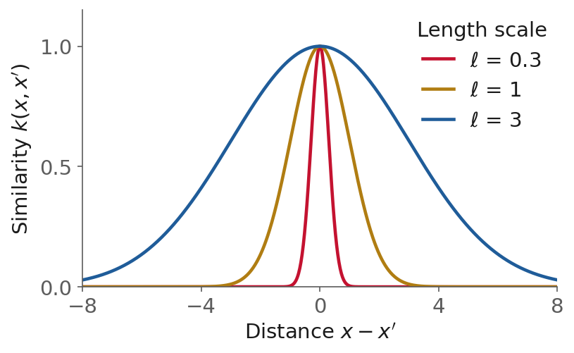
Fig. 44 The RBF (squared exponential) kernel: similarity falls with distance, and the length scale sets how fast.

The kernel’s hyperparameters are the length scale \(\ell\) (how far apart two inputs can be and still be correlated), the signal variance \(\sigma_f^2\) (the output scale) and the noise variance \(\sigma_n^2\). They play a role analogous to a neural network’s architecture and regularization choices.

Training. The kernel hyperparameters are not set by hand: .fit chooses them by solving an optimization problem, which the end of this section writes out.

An example. Back to the surfactant data from the examples section, on log axes. Scaling is important for kernels, just as it is for the activations in a neural network, so we standardize \(x\), and scikit-learn optimizes the kernel hyperparameters for us:

from sklearn.gaussian_process import GaussianProcessRegressor
from sklearn.gaussian_process.kernels import RBF

gpr = GaussianProcessRegressor(
    kernel=RBF(length_scale=1.0),
    alpha=0.1,
    normalize_y=True,
    n_restarts_optimizer=5,
)
gpr.fit(X_train_scaled, y_train)
y_mean, y_std = gpr.predict(X_grid_scaled, return_std=True)

The fitted RBF length scale is 0.235 in standardized units, and the model scores \(R^2 = 0.783\) on the four test points. Swapping the kernel for a Matérn with \(\nu = 3/2\) plus a white-noise term scores 0.836.

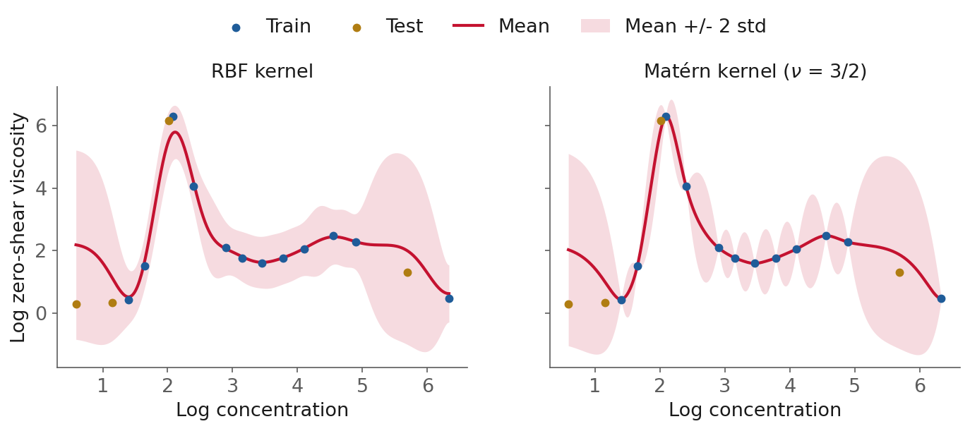
Fig. 45 Gaussian process regression on the surfactant data, with an RBF kernel (left) and a Matérn kernel with \(\nu = 3/2\) plus white noise (right). The band is the mean plus or minus two standard deviations.

Strengths and weaknesses. GPs give flexible, probabilistic predictions with an uncertainty attached, their kernels can be designed and interpreted, and the marginal likelihood gives an automatic Occam’s razor. On the other side, they scale as \(\mathcal{O}(N^3)\) and are expensive for large \(N\) (sparse and approximate GPs exist for that), the kernel choice matters, because it is the model’s inductive bias, and they need careful scaling and validation.

What its training solves. It is the same template as the network’s, with different decision variables and a different objective:

\[ \begin{aligned} \text{Neural network:} \quad \min_{W,\,b} \quad & \sum_{i=1}^{N} \big(y_i - f(x_i; W, b)\big)^2 \end{aligned} \]

\[\begin{split} \begin{aligned} \text{Gaussian process:} \quad \min_{\boldsymbol{\theta}} \quad & -\log p(\mathbf{y} \mid X, \boldsymbol{\theta}), \qquad \boldsymbol{\theta} = \log(\sigma_f^2, \ell, \sigma_n^2) \\ \text{s.t.} \quad & \log 10^{-5} \le \theta_j \le \log 10^{5} \end{aligned} \end{split}\]

The network’s variables are its weights and biases (10 in the three-unit model, 161 in the concrete network), and its objective is the squared error. They are free: scikit-learn’s lbfgs solver calls SciPy’s L-BFGS-B routine with no bounds at all, which makes it plain L-BFGS, and Adam and SGD apply none either. A Gaussian process has no weights. Its decision variables are the handful of kernel hyperparameters, and in scikit-learn the bounds are real constraints: every kernel carries bounds for its hyperparameters, and GaussianProcessRegressor hands them to the same L-BFGS-B routine. It works on the logarithms of the hyperparameters, \(\boldsymbol{\theta} = \log(\sigma_f^2, \ell, \sigma_n^2)\), because length scales and variances naturally live on a log scale, so the constraints are bounds on those logarithms. The alpha added to the diagonal is not optimized; the noise is learned only through a WhiteKernel term. Other libraries reach the same end without bounds: GPflow and GPyTorch keep each hyperparameter positive by passing an unconstrained raw value through a softplus transform, and optimize the raw values freely, with L-BFGS-B in GPflow and with Adam in GPyTorch’s examples. The RBF kernel’s default bounds on its length scale are \(10^{-5}\) and \(10^{5}\), and n_restarts_optimizer restarts the optimizer from points drawn log-uniformly inside the bounds, a multistart that any process systems engineer would recognize. A note on words: scikit-learn calls \(\ell\), \(\sigma_f\) and \(\sigma_n\) hyperparameters, and yet .fit optimizes them. For a Gaussian process they play the part that the weights play in a network. What stays fixed before training, and is a hyperparameter in Lecture 8’s sense, is the choice of kernel and its bounds.

Start from the model. The measurements are a smooth function plus noise, \(y = f(x) + \varepsilon\), with a GP prior \(f \sim \mathcal{GP}(0, k_\theta)\) and Gaussian noise \(\varepsilon \sim \mathcal{N}(0, \sigma_n^2)\). Averaging over every function \(f\) the prior allows, the vector of measurements is itself Gaussian, \(\mathbf{y} \sim \mathcal{N}(\mathbf{0}, K_\theta + \sigma_n^2 I)\). The marginal likelihood is the probability of the data you measured under that distribution, with \(f\) “marginalized”, that is, averaged out. Training maximizes it, which is the same as minimizing its negative logarithm, and that has three terms:

\[-\log p(\mathbf{y}\,|\,X,\theta) = \underbrace{\tfrac{1}{2}\mathbf{y}^\top(K_\theta+\sigma_n^2 I)^{-1}\mathbf{y}}_{\text{misfit}} \;+\; \underbrace{\tfrac{1}{2}\log\det(K_\theta+\sigma_n^2 I)}_{\text{complexity penalty}} \;+\; \underbrace{\tfrac{N}{2}\log 2\pi}_{\text{constant}}.\]

This automatically balances the fit to the data (the first term) against the model’s complexity (the log-determinant term); \(N\) is the number of points, and the constant does not change the optimum. In plain terms: the misfit is small when the kernel explains the measurements well. The complexity penalty charges for flexibility. Minimizing the sum of these picks the simplest model that still explains the data, which is Occam’s razor somewhat represented as an objective.

The length scale is the hyperparameter that trades the two terms most visibly. It sets how far apart two inputs can be and still be correlated. A short length scale lets the function change between neighboring points; a long one forces it to be smooth over the whole range. Here is the trade-off on the surfactant data. For this figure the GP is refitted on all 16 points with a signal variance and a white-noise term, the full problem written above, and then the signal variance and the noise are held at their fitted values while only the length scale changes. That refit is why its length scale differs from the 0.235 of the example above, which used 12 training points, standardized inputs, and a noise fixed by alpha=0.1.

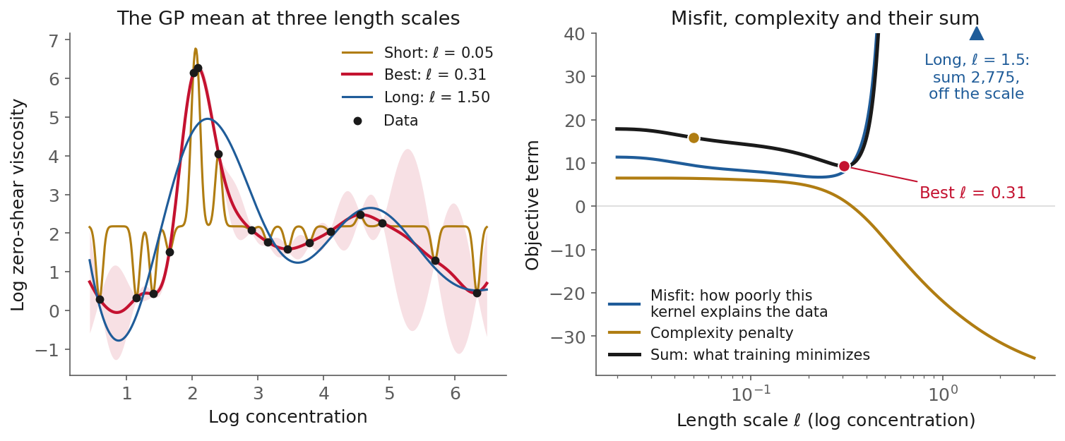
Fig. 46 The length-scale trade-off on the surfactant data, with the signal variance and the noise held at their fitted values. Left: the GP mean at a short, the best and a long length scale. Right: the misfit, the complexity penalty and their sum, which training minimizes, against the length scale.

The complexity penalty is what rules out the short length scale: it is 6.43 at \(\ell = 0.05\) against 1.31 at the best value, while the misfit moves much less (9.42 against 7.94). The long length scale is ruled out by the misfit: a curve that smooth cannot reach the peak, and the misfit climbs to 2,803. The sum is smallest at \(\ell = 0.31\) in units of log concentration, which is the length scale of the refit on all 16 points (0.19 in standardized units, the same value).

Notice what is not optimized: the prediction itself. Given the hyperparameters, the predicted mean and variance are the linear algebra from the GP section, a solve with \(K + \sigma_n^2 I\). So a GP’s training is a small non-convex problem with few variables (the concrete GP has ten: a length scale for each of the eight inputs, a signal variance and a noise level). Every evaluation of its objective, though, factorizes an \(N \times N\) matrix, at a cost of \(\mathcal{O}(N^3)\) (a very computationally expensive operation). The same cost limits the GP-NARX below with respect to the number of data points used. The problem is non-convex too, which is why n_restarts_optimizer starts the optimizer from several points and keeps the best.

What each model optimizes

With all four model families introduced, here is what each .fit solves, side by side.

Model	Decision variables	Objective	Kind of problem	How it is solved
Linear regression	Coefficients \(a\)	\(\sum (y_i - a^\top x_i)^2\)	Convex quadratic, one minimum	One least squares solve
Ridge and lasso	Coefficients \(a\)	The same, plus \(\alpha \sum a_i^2\) or \(\alpha \sum \lvert a_i \rvert\)	Convex (the lasso is not smooth)	One solve (ridge), coordinate descent (lasso)
Decision tree	The splits	Squared error, one split at a time	Combinatorial	Greedy search
Neural network	Weights and biases \(W, b\)	\(\sum (y_i - f(x_i; W, b))^2\)	Non-convex, many local minima	L-BFGS, Adam, stochastic gradient descent
Gaussian process	Kernel hyperparameters \(\ell, \sigma_f, \sigma_n\)	\(-\log p(\mathbf{y} \mid X, \theta)\)	Non-convex, few variables, bounded	L-BFGS-B, from several starting points

Linear regression is the easy case. Its loss is a convex quadratic in the coefficients, so it has one minimum, and least squares finds it in one linear solve from any starting point; that is the lstsq of Lecture 7. Everything below it in the table needs an iterative method or a search.

Back to Lecture 8: NARX with a network and a GP

Nothing in the four models needs the rows to be separate experiments. Lecture 7 built a NARX table, where each row holds past values of a channel and of its inputs and the target is a later value, and Lecture 8 fitted a linear model to it as a direct forecaster. Hand the same table to a network or a GP and you have an NN-NARX or a GP-NARX, with the same fit and predict.

Take Lecture 8’s table exactly. The target is the reactor pressure \(y\) (the channel xmeas_7) 30 minutes ahead, and the inputs are its last ten values, one every three minutes, and the eleven valve positions \(u_1, \dots, u_{11}\) now:

\[ \hat{y}(t + 30\,\text{min}) = f\big(y(t),\, y(t - 3),\, \dots,\, y(t - 27),\; u_1(t),\, \dots,\, u_{11}(t)\big), \]

with times in minutes. When \(f\) is linear, as in Lecture 8’s ridge fit, this is an ARX model; when \(f\) is a network or a GP, it is a NARX model, a nonlinear ARX. Train on fault-free runs 1 to 300 (144,300 rows) and test on runs 401 to 500, which is Lecture 8’s split by run.

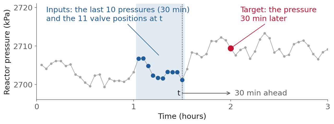
Fig. 47 One row of the NARX table on a real run: the inputs are the last 30 minutes of pressure and the valve positions at \(t\), and the target is the pressure 30 minutes later.

from sklearn.compose import TransformedTargetRegressor

nn_narx = TransformedTargetRegressor(          # scale the target, not only the inputs
    regressor=make_pipeline(
        StandardScaler(),
        MLPRegressor(
            hidden_layer_sizes=(32,),
            activation="tanh",
            solver="adam",
            max_iter=500,
            early_stopping=True,
            random_state=0,
        ),
    ),
    transformer=StandardScaler(),
)
gp_narx = make_pipeline(
    StandardScaler(),
    GaussianProcessRegressor(
        kernel=kernel,
        normalize_y=True,
    ),
)

Model	Training rows	Test RMSE (kPa)
Baseline: persistence	None	5.82
Baseline: predict the mean	None	7.57
ARX, ridge with \(\alpha = 1\) (Lecture 8)	144,300	4.71
NN-NARX, 32 tanh units	144,300	4.73
NN-NARX, target not scaled	144,300	7.57
GP-NARX	1,000	4.76
ARX on the same 1,000 rows	1,000	4.76

Two things come out of the table. First, scale the target as well as the inputs. Reactor pressure sits near 2,705 kPa with a standard deviation of 7.7 kPa, so an unscaled network has to produce 2,705 from weights that start near zero, and this one stopped at the mean: 7.57 kPa, exactly the score of predicting the mean. TransformedTargetRegressor with a StandardScaler fixes it, and the GP’s normalize_y=True does the same job. It is a similar idea to Lecture 7’s deviation variables.

Second, the nonlinear models tie the linear one. Held at its operating point the plant behaves close to linearly (Lecture 7 fitted this loop as a first-order process), so a network and a GP have nothing extra to find, and on the same 1,000 rows the GP and a ridge ARX both score 4.76 kPa. What the GP adds is a band: 94.8% of the test measurements fall within two of its predicted standard deviations.

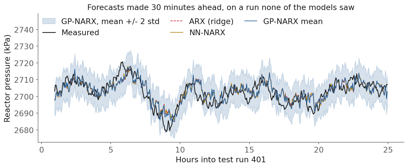
Fig. 48 Thirty-minute forecasts of reactor pressure on a test run, from the linear ARX, the NN-NARX and the GP-NARX, with the GP’s band.

The four model families on the concrete strength dataset

Now the main example. Here are the four models on the 835 training rows of the concrete data, scored by five-fold cross-validation with the rows assigned to the folds at random. The folds are the subject of the next section. The neural network has 16 tanh units, and the GP has one RBF length scale per input plus a white-noise term; both see standardized inputs.

Model	RMSE (MPa)	MAE (MPa)	\(R^2\)
Baseline: predict the mean	16.8	13.6	−0.01
Linear	10.6	8.46	0.60
Linear, with physics features	7.25	5.60	0.81
Decision tree (no depth limit)	6.92	4.52	0.83
Neural network	5.96	4.20	0.87
Gaussian process	5.81	3.96	0.88

The first row is a baseline, as in Lecture 8: the score of a model that ignores every input and predicts the training mean, which any real model has to beat. The physics features are the logarithm of the age and the water-to-cement ratio, from the section on linear regression. Read this way, the flexible models win, the tree beats the engineered straight line, and the network and the GP are nearly tied. Keep that ranking in mind: the section on cross-validation shows how much of it comes from the way the rows were split.

Choosing a model with cross-validation

k-fold cross-validation

A single validation split gives a noisy answer, and it sets part of the data aside for checking only. Cross-validation uses every row for both.

Definition: k-fold cross-validation

k-fold cross-validation splits the training data into \(k\) parts (folds), trains \(k\) times while holding out a different fold for validation each time, and averages the \(k\) validation scores. Every row is used for validation exactly once.

The figure plots which rows belong to training and which to validation in each fold, for 30 rows and five folds.

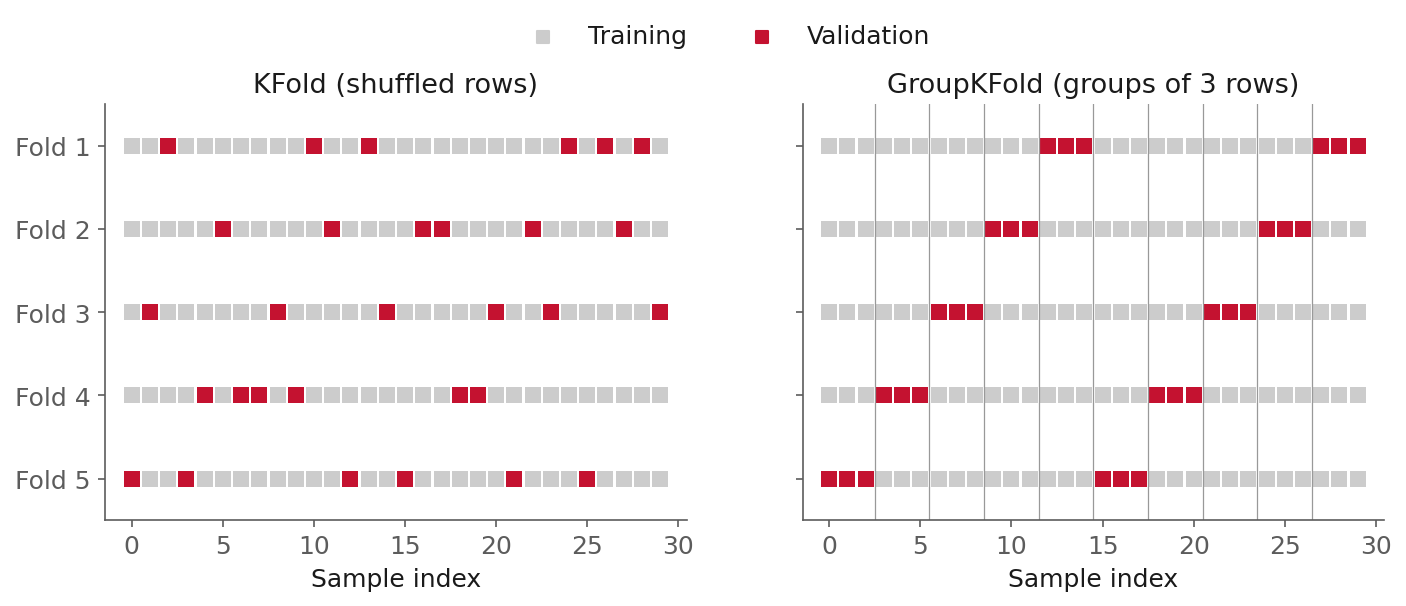
Fig. 49 Five folds over 30 rows. Left: KFold with shuffling assigns rows at random. Right: GroupKFold with groups of three rows keeps every group together.

In scikit-learn, cross-validation is one call. scikit-learn always maximizes scores, so errors come back negative:

from sklearn.model_selection import KFold, cross_val_score

cv = KFold(
    n_splits=5,
    shuffle=True,
    random_state=0,
)
scores = cross_val_score(
    model, X_train, y_train,
    cv=cv,
    scoring="neg_root_mean_squared_error",
)
print(-scores.mean(), scores.std())

Report the spread across the folds next to the mean. On concrete, the fold-to-fold standard deviation of the GP’s RMSE is about 0.7 MPa, so two models 0.3 MPa apart are tied.

Grouped rows: GroupKFold

The 428 mixes from the examples section are where this comes from. Group the 1,030 rows by their seven ingredient amounts, ignoring the age, and they collapse into 428 distinct mixes. 182 of those mixes were crushed at more than one age (3, 7, 28, 56, 90 days, and so on), and between them they hold 76% of the rows. 25 rows are exact copies of another row. A random KFold puts the 28-day row of a mix in the training folds and the 56-day row of the same mix in the validation fold, so the model is asked about a mix it has already seen at another age. That is an easier question than the one an engineer asks, which is how strong a mix nobody has made yet will be.

Definition: grouped cross-validation

Grouped cross-validation (GroupKFold in scikit-learn) assigns whole groups to folds, so that all the rows of a group (one mix, one batch, one specimen, one run) are either all in training or all in validation.

Lecture 8 did this for simulation runs, where it was called splitting by series. Nothing about it needs a time axis: whenever rows share a physical unit, the unit is what you hold out.

from sklearn.model_selection import GroupKFold

MIX = ["cement", "slag", "fly_ash", "water", "superplasticizer", "coarse_agg", "fine_agg"]
mix = df.groupby(MIX).ngroup().to_numpy()   # one integer per distinct mix
mix_train = mix[train]                      # train: the rows kept when the test mixes were locked
scores = cross_val_score(
    model, X_train, y_train,
    cv=GroupKFold(n_splits=5),
    groups=mix_train,
    scoring="neg_root_mean_squared_error",
)

The figure makes the difference concrete on six real mixes, each crushed at 3, 7, 28 and 90 days.

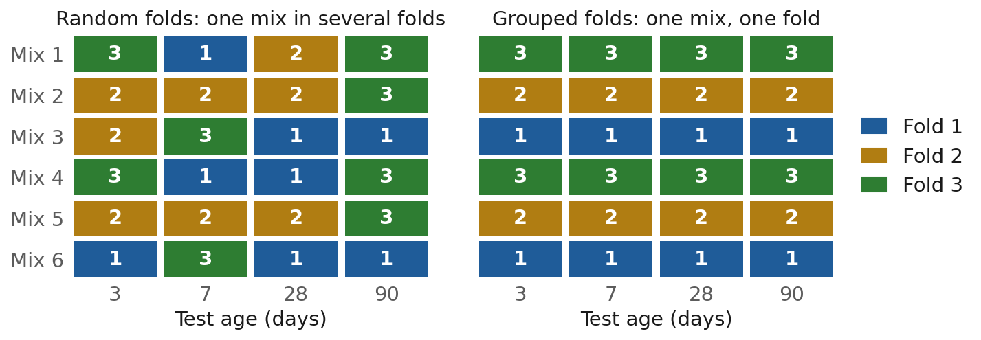
Fig. 50 Folds of rows against folds of mixes, for six mixes (three folds, for legibility). Random folds scatter the ages of one mix across folds; grouped folds keep each mix in one fold.

The test set was locked the same way, by mix. Here are the same models scored both ways.

Fig. 51 Five-fold cross-validated RMSE on the 835 training rows, with random folds (gray) and folds of whole mixes (red). Error bars are the standard deviation across the five folds.

Model	KFold RMSE (MPa)	GroupKFold RMSE (MPa)
Baseline: predict the mean	16.8	16.8
Linear	10.6	10.7
Linear, with physics features	7.25	7.43
Decision tree	6.92	9.42
Neural network	5.96	8.02
Gaussian process	5.81	7.17

The baseline and the two linear models barely move, because none of them can memorize a mix. The flexible models all get worse, and the tree gets worse the most (by 36%), because a tree with no depth limit is the best of the four at memorizing. The ranking changes too. Under random folds the tree beats the engineered straight line; under folds of whole mixes it loses to it by 2 MPa, and the straight line, with its two features from a century of concrete engineering, is within 0.3 MPa of the GP.

What a practitioner should take from this

Before you choose a splitter, ask what one independent experiment is in your data: a mix, a batch, a specimen, a run, a patient. Count the rows per unit. If a unit has more than one row, split by unit with GroupKFold, for the test set as well as the folds, and expect the flexible models to lose more than the simple ones. The gap between KFold and GroupKFold on your data tells you how much your models were memorizing.

Model capacity, overfitting and learning curves

Every model in this session has a “knob” that sets how flexible it is: the degree of the polynomial, the depth of a tree, the number of hidden units, the penalty \(\alpha\), the length scale of a kernel. This section is about turning that knob, and about the two curves that tell you which way to turn it.

Capacity, underfitting and overfitting

Definition: model capacity

The capacity of a model is the range of functions it can represent. More capacity lets it fit more complicated relationships, and also more of the noise.

Overfitting is a common issue in ML. It occurs when the model works extremely well on the training data, but it does not generalize well when we make predictions on the validation or test sets. Underfitting is the opposite failure.

Definition: overfitting and underfitting

A model overfits when its training error is much lower than its validation error: it has fit the noise and the particular rows it was given. It underfits when both errors are high and close together: it is too simple to represent the relationship.

Bias and variance

The expected squared error of a model at an input \(x_0\) splits into three parts (Hastie, Tibshirani and Friedman, section 7.3, equation 7.9):

\[ \text{Err}(x_0) = \sigma^2_\varepsilon + \text{Bias}^2\big(\hat f(x_0)\big) + \text{Var}\big(\hat f(x_0)\big) \]

The first term is the noise in the measurement itself, which no model can remove. The second is the squared bias, how far the model’s prediction is from the truth on average, over the training sets you could have drawn. The third is the variance, how much the prediction moves when the training set changes. In the book’s words, “typically the more complex we make the model \(\hat f\), the lower the (squared) bias but the higher the variance.”

Definition: bias-variance trade-off

The bias-variance trade-off is that adding capacity lowers a model’s bias (its systematic error) and raises its variance (its sensitivity to the particular training rows), so the validation error is lowest at some capacity in between.

On concrete, a straight line is the high-bias end: however many mixes you give it, it cannot bend to the data. A tree with no depth limit is the high-variance end: change a few training mixes and its leaves change with them. Regularization is a knob on the same axis, trading a little bias for less variance.

Validation curves: error against capacity

Definition: validation curve

A validation curve plots the training error and the validation error against one capacity knob (a hyperparameter), with the data held fixed.

Let’s go straight to an example. We increase the capacity through the max_depth of a decision tree on concrete, and track the training RMSE and the validation RMSE.

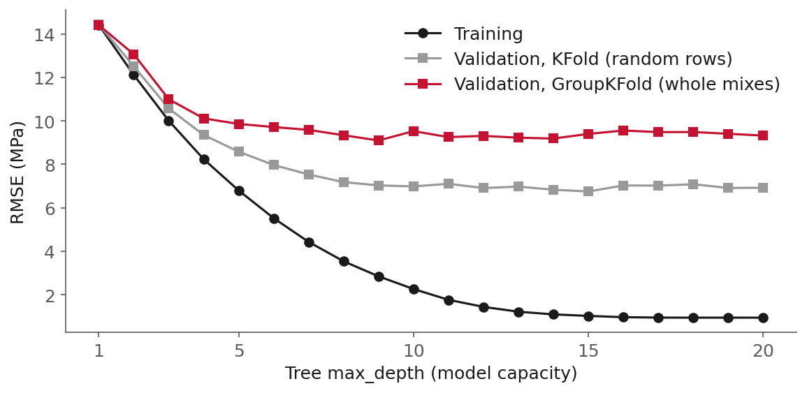
Fig. 52 Training and validation RMSE for trees of increasing depth on the 835 concrete training rows. The gray curve uses random folds and the red curve uses folds of whole mixes.

The training RMSE keeps falling as the tree deepens, from 14.4 MPa at depth 1 to 0.95 at depth 17 and beyond. The validation RMSE under GroupKFold stops improving at depth 9 (9.10 MPa) and wobbles between 9.2 and 9.6 after that. Looking only at the training score can be misleading! The training error never reaches zero, either. Nine settings in the file (the same mix at the same age) were crushed more than once and gave different strengths. One of them gave anywhere from 22.9 to 55.9 MPa at 7 days. No model can give two answers to the same input, so this is the noise term of the decomposition, made visible. The gray curve is the same sweep under random folds. It keeps improving, down to 6.8 MPa, because a deeper tree memorizes more mixes, and random folds reward memorizing.

from sklearn.model_selection import validation_curve

train_scores, valid_scores = validation_curve(
    DecisionTreeRegressor(random_state=0), X_train, y_train,
    param_name="max_depth",
    param_range=range(1, 21),
    cv=GroupKFold(5),
    groups=mix_train,
    scoring="neg_root_mean_squared_error",
)

Learning curves: error against data

Definition: learning curve

A learning curve plots the training error and the validation error against the number of training samples, with the model held fixed.

It answers a question that no single score can: would more data help?

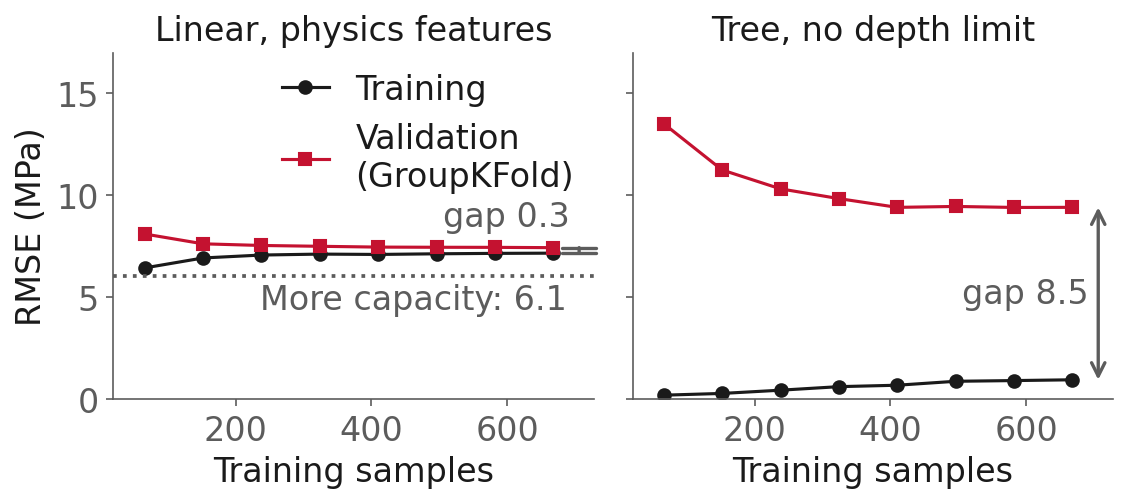
Fig. 53 Learning curves on concrete with folds of whole mixes, for linear regression with physics features (left) and a tree with no depth limit (right). Each curve is the mean over ten random orderings of the training rows. The dotted line is gradient-boosted trees given the same features and scored on the same folds, a model with more capacity than the line.

Read two things off each panel. The first is the gap between the two curves at the right edge. It measures variance: how much worse the model does on samples it was not fitted to than on the samples it was. The second is the level where the curves end up, which measures bias, plus the noise that no model can remove.

The engineered straight line has almost no gap. With 668 training samples its training RMSE is 7.16 MPa and its validation RMSE 7.43, and the gap shrank to 0.3 MPa as the training set grew. The line therefore no longer overfits, and more samples can close at most the 0.3 MPa that is left.

Curves that meet at a level another model can beat are the signature of underfitting, or high bias: the model is too simple for the relationship, and more training samples will not help it. The actions are more capacity or better features.

The tree model has the opposite shape: 0.95 MPa on its training samples and 9.42 on validation, a gap of 8.5 MPa, which is overfitting, or high variance. Its validation curve is flat near 9.4 MPa from about 400 samples on, so more samples of the same kind are not closing the gap. Capping the depth is the other lever, and the validation curve above shows it buys little here: the best depth, 9, reaches 9.10 MPa.

Shuffle the rows before you draw a learning curve. To build each smaller training set, learning_curve takes the first rows of the fold in the order they appear in the file, unless you pass shuffle=True. The concrete file is not in random order, so those first rows are not a fair sample of the rest. Without shuffling, the tree’s validation error dropped by 3.5 MPa near the right edge only because a new block of rows entered the training set, and the curve seemed to say that more data would help. With the rows shuffled, the same curve is flat from about 400 samples on.

from sklearn.model_selection import LearningCurveDisplay

LearningCurveDisplay.from_estimator(
    model, X_train, y_train,
    cv=GroupKFold(5),
    groups=mix_train,
    scoring="neg_root_mean_squared_error",
    negate_score=True,
    shuffle=True,
    random_state=0,
)

Reading the two curves

What the curves show	Diagnosis	What helps	What does not
Training and validation error both high, and close together	Underfitting (high bias)	More capacity, better features	More data
Training error low, validation error much higher	Overfitting (high variance)	Less capacity, regularization, more data	More capacity
Validation error still falling at the largest training size	Limited by data	More data
Training and validation error both low, and close together	A good fit	Stop here, and test once	More tuning

The first and last rows have the same shape, two curves that meet, and they differ only in the level. So a closed gap tells you only that more data will not lower the error; the level tells you whether the model is good. On concrete the engineered line sits in the first row, and the unlimited tree in the second. Read the curves before you change the model, because the two diagnoses call for opposite actions.

Choosing, then testing once

Of the four model families this session teaches, the GP has the lowest grouped validation error (7.17 MPa), so it is the one tested here. The boosted trees from the learning-curve section scored a bit lower (6.06 MPa) and beat the GP on all five folds. On a project of your own that score would make them the model to test. Since we are not looking into boosted trees, we won’t expand the discussion here. Instead, we fit the GP on all 835 training rows and score the 86 held-out mixes, once.

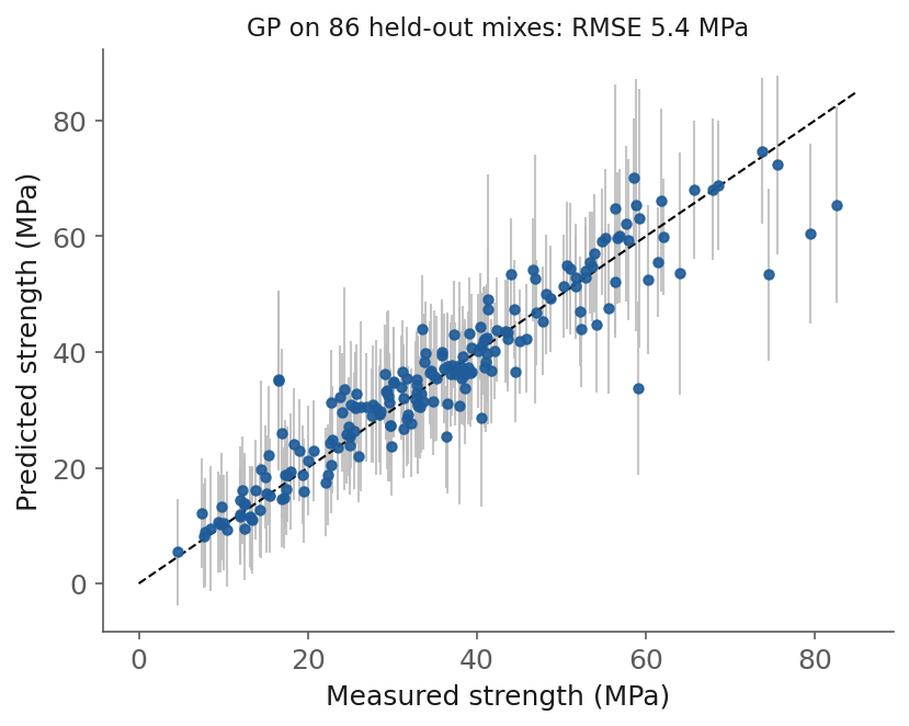
Fig. 54 The chosen model, tested once. Each bar is the GP’s prediction plus or minus two of its own predicted standard deviations.

The test RMSE is 5.39 MPa, the MAE 3.72 and \(R^2 = 0.889\). That is lower than the 7.17 the folds predicted, and the difference is sampling noise: 86 mixes are one draw, and across ten other random draws of the test mixes the same GP scores between 5.45 and 7.42 MPa. A test number carries its own uncertainty, and a test set of a couple of hundred rows can move by a megapascal or two in our case here. The GP also reports a standard deviation for each prediction, 5.2 MPa on average, and 95.4% of the test points fall within two of them.

Limitations

Every model in this session is fitted to the region its data covers, and each model fails in its own way outside it.

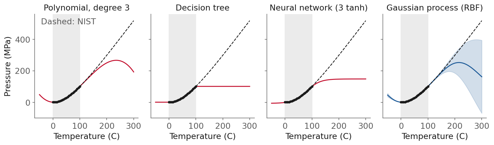
Fig. 55 Four models fitted on the same 21 water points between 0 and 100 °C, then asked about −50 to 300 °C. The dashed line is NIST, which none of them saw beyond 100 °C.

We fit all four models on the 21 water points between 0 and 100 °C and ask them about 300 °C, where NIST gives 517.7 MPa. The third-degree polynomial bends over and answers 192 MPa (not the 223 MPa of the opening, because this one is fitted on all 21 points rather than 16). The tree cannot predict anything outside the range of its training targets, so it stays flat at its last leaf, 100.7 MPa. The network’s tanh units saturate, and it levels off at 148 MPa. The GP’s mean turns back toward the average of its training data (it reads 162 MPa at 300 °C), and its uncertainty band grows, to plus or minus 232 MPa. The band still misses the truth. A GP’s uncertainty describes how far a point is from the data, under the kernel’s assumption about smoothness; it says nothing about physics the data never showed it.

Where scikit-learn stops

The Gaussian process also shows where this session’s tools stop. The NN-NARX trained on all 144,300 rows of Lecture 8’s table in about 2 seconds. The GP-NARX got 1,000 of them and took about half a minute; with 4,000 rows it took about 6 minutes and improved to 4.72 kPa, which the ridge ARX on the same 4,000 rows matched. All 144,300 rows would need a 144,300 by 144,300 kernel matrix, roughly 167 GB in space, before a single solve.

scikit-learn is built for data that fits in the memory of one PC/machine. It runs on the CPU, and its models are a fixed catalog: its networks do train with Adam on mini-batches, but you cannot write a model of your own and have its gradients computed for you. Data at plant scale, and models with millions of parameters, need the stochastic rows of the optimization section’s table run on GPUs, with the gradients of any model you write from automatic differentiation. Those are what PyTorch and JAX, the machine learning tools in the course syllabus, provide. The ideas in this session carry over to them unchanged.

But wait, we didn’t discuss the hyperparameters?

Look back at the choices this session made by hand: 16 hidden units, a tree with no depth limit, the kernel’s forms of the GP section, and the decision tree hyperparameter. None of them was fitted, or determined systematically. In the language of the optimization section, they are not decision variables of the training problem. Instead, they are fixed before it is solved. Choosing them well is an optimization problem too, one level up:

\[\begin{split} \begin{aligned} \min_{\lambda} \quad & L_{\text{val}}\big(\theta^*(\lambda)\big) \\ \text{s.t.} \quad & \theta^*(\lambda) = \arg\min_{\theta} \; L_{\text{train}}(\theta; \lambda) \end{aligned} \end{split}\]

where \(\lambda\) holds the hyperparameters. It is an optimization problem with another optimization problem inside it: every evaluation of the outer objective means training a model, and the validation data now does double duty, since the best of many validation scores is an optimistic number. How do you search over \(\lambda\) without training thousands of models, and without fooling yourself with the winner’s score? This session leaves that question open.

Worked example

The notebook l09-regression.ipynb is a worked example, and it is not run in class. Run it yourself after the session, top to bottom: it walks through the concrete workflow and the NARX forecasts from the slides, one step per cell, on the real data. It downloads the concrete data from UCI (125 kB) and the fault-free Tennessee Eastman file (25 MB) on its first run, and the cross-validation cell takes a minute or two. It follows the concrete sections of these notes first, then Lecture 8’s NARX table:

1. Concrete. Lock a test set of whole mixes, then fit the mean, the linear models, the tree, the network and the GP with the same fit and predict.

2. Two splitters. Score every model under KFold and under GroupKFold, and watch the ranking change.

3. Test once. Fit the chosen model on all the training rows, and score the held-out mixes.

4. NARX. Lecture 8’s pressure table, fitted with a ridge ARX, an NN-NARX and a GP-NARX.

Summary

Every supervised model in scikit-learn is created, fitted and scored the same way, so what decides the result is the split, the features and the metric. The concrete data showed the split at work. With rows assigned to folds at random, a decision tree beat a straight line given two physics features; with whole mixes held out, the tree lost to that line by just 2 MPa, and the line came within 0.3 MPa of a Gaussian process.

Under every model is an optimization problem: least squares for a line, a greedy search for a tree, a non-convex problem over weights and biases for a network, and a bounded problem over a few kernel hyperparameters for a Gaussian process, with the iterative ones solved by L-BFGS when a full gradient is cheap and by stochastic methods such as Adam when it is not.

No model wins everywhere, which is why the session compared four of them, on a table of experiments and on Lecture 8’s plant table, and why validation, not preference, chooses between them.

None of the four can be trusted outside the data it was fitted to: at 300 °C every one of them missed the water pressure, and the Gaussian process’s band missed with it. Reading the validation and learning curves before changing a model tells you which way to change it, because underfitting and overfitting call for opposite actions.

Resources

• Victor Alves, 06-325 Numerical Methods and Machine Learning for Chemical Engineers (Fall 2025), lectures 6 to 10. The undergraduate version of this session, with the water, network and GP examples worked step by step; the notebooks and data are in the course repository.

• Hastie, Tibshirani and Friedman, The Elements of Statistical Learning, chapter 7. Interesting material regarding cross-validation.

• The scikit-learn User Guide, cross-validation.

• The scikit-learn User Guide, metrics and scoring. What each metric computes.

• The scikit-learn User Guide, linear models, decision trees, neural network models and Gaussian processes. The four models, each with its options and its practical tips.

• The scikit-learn User Guide, validation and learning curves. validation_curve and LearningCurveDisplay.

• Rasmussen and Williams, Gaussian Processes for Machine Learning (MIT Press, 2006). The GP book, free online. Chapter 2 derives the predictive mean and variance used above.

• A Visual Exploration of Gaussian Processes, Distill (2019). Interactive: move the training points and change the kernel, and watch the posterior respond.

• David Duvenaud, The Kernel Cookbook. What functions drawn from each kernel look like, and how sums and products combine them.

• 3Blue1Brown, Neural networks, a video series with animations of what a network computes and how it trains.

• Liu and Nocedal (1989), On the limited memory BFGS method for large scale optimization, Mathematical Programming 45, 503 to 528 (paywalled; the author copy is free). L-BFGS, the solver behind most small-data fits in this session. The math behind training of ML models.

• Kingma and Ba (2015), Adam: A Method for Stochastic Optimization

• Bottou, Curtis and Nocedal (2018), Optimization Methods for Large-Scale Machine Learning, SIAM Review 60(2) (the arXiv copy is the authors’). Stochastic and batch methods compared from the optimization side; section 3 defines both.

• The no free lunch theorem for supervised learning: Wolpert’s 2020 overview of the theorems is free.

• Yeh (1998), Modeling of strength of high-performance concrete using artificial neural networks, Cement and Concrete Research 28(12), 1797 to 1808 (paywalled). The origin of the concrete data, which is on UCI under CC BY 4.0.

• SysIdentPy, a Python library for system identification with NARMAX models. It selects which lagged terms enter a polynomial NARX, and it also wraps neural and scikit-learn models as NARX.

• Downs and Vogel (1993), A plant-wide industrial process control problem, TEP original source, the original simulation code is free and lists the 20 disturbances in its header.

• Rieth, Amsel, Tran and Cook (2017), Additional Tennessee Eastman process simulation data. The source of both plant files; the fault list is in the header of teprob.f.

• Prof. Kitchin’s Data science and machine learning in science and engineering and Prof. Ulissi’s Numerical Methods and ML for ChE notes (CC BY 4.0). Two CMU courses that cover the same models from different angles.

Assignment

No assignment is released today.

Practice module

Practice module for this session.