Lecture 7: Features for time-series models

At a glance

• Session Lecture 7, Week 4

• Arc Data Systems

• Slides Deck for this session

• Practice Practice module for this session

• Demo l07-timeseries.ipynb, building and solving an ARX regressor matrix

• Tools Polars for the table (same as Lecture 5), numpy.linalg.lstsq for the fit

• No Assignment today. Assignment A4 is released at the next lecture.

Why this matters

Today we look at features for time-series data: which columns belong in the table when the rows came from a process that changes over time.

That is most of the data a chemical engineer works with. A few examples:

• Process control: a flow responding to the valve that sets it.

• Reaction kinetics: a concentration falling through a batch.

• Plant historians: every instrument on a unit, logged every few minutes, for years.

• Fault detection: a channel that starts to drift long before it alarms.

The same table problem shows up well outside chemical engineering:

• Mechanical: a bearing’s vibration, where wear accumulates and never resets.

• Power systems: a battery’s state of charge, which is the integral of everything you have drawn from it.

• Buildings: a thermostat chasing a temperature setpoint, with the walls in between.

• Infrastructure: a request queue, whose length now depends on how long it already was.

• Biomedical: a drug concentration decaying between doses.

• Demand and capacity planning: tomorrow’s load from today’s, where shuffling the rows into a random train/test split quietly lets the model read the future.

All of them share one property. What you measure now depends on what the system was “doing” before, and not only on the inputs right now. A table that carries only the current inputs will be missing this information.

The last one (Demand and capacity planning) is different. Every other example is a physical system with something stored in it: heat, charge, mass, damage, queued work. A demand series has no such store. A model of it still fails in the same ways a plant model does.

How would you know your feature table is right?

Feature engineering has one difficulty above all others. You build a table, fit a model, and it reports an R-squared of 0.94. That number is just as high for a table that quietly used a future value, or grouped on the wrong column, or leaned on a sensor that was only repeating its last reading. The score cannot “catch” any of those mistakes.

So we work one concrete problem all class, chosen because its answer is checkable, for our learning purposes.

We use a feed stream from the TEP process: a valve, and the flow it sets. The process behind it is first order, which means the two coefficients a fit returns convert into a time constant in minutes and a gain in flow per percent of valve. Those are physical quantities with units. In this specific case, a plant engineer who knows that line can tell you whether ten minutes is credible for it. Nobody can tell you whether an R-squared is credible immediately.

That gives us a feature table we can check, and it is the one of the few places in this course where a model’s output can be checked against physics rather than against another number from the same data. Everything else today is about building that table correctly.

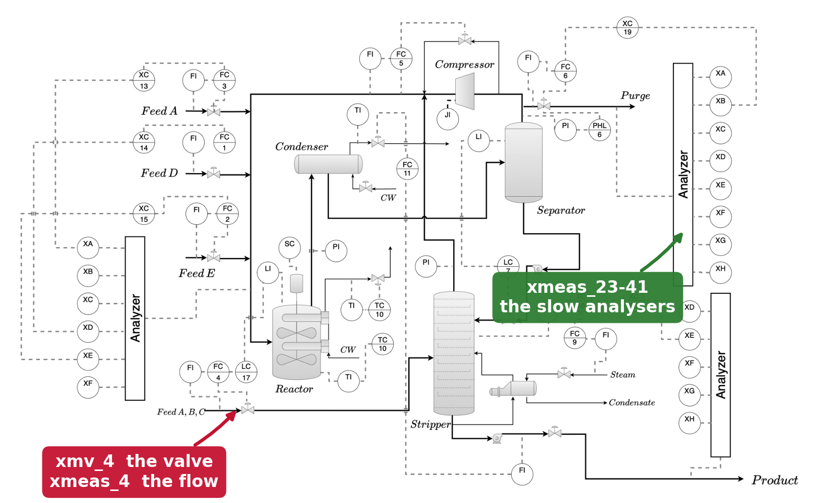
Fig. 14 The plant, with the two channel families this session touches. Everything today happens at the valve marked on the lower left. The analyser blocks come back at the end, when we screen the channels. P&ID from Lyu, Botcha, Kulkarni, Pagaria, Alves, Sunshine and Kitchin (2026).

There is a second benefit. The textbook way to get a time constant is a step test: move the valve, wait for the measurement to settle, read the response off the chart. Try scheduling one. A step test means asking operations to take a production unit off its setpoint so you can watch it drift. Meanwhile the plant has logged that same loop every three minutes for years, and nobody had to approve anything.

The logged data has a problem

Plot the measurement against the valve and you get a cloud, not the tidy line a step test gives you.

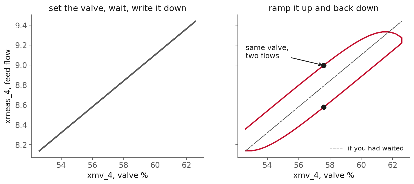
Fig. 15 The A and C feed loop of the Tennessee Eastman Process (TEP), run two ways. Set the valve and wait, and every point is a settled state on a line. Ramp it without waiting and the points fall on a loop: at 57.6 % the flow is 8.578 going up and 8.997 coming down. Both panels are simulated, at the time constant and gain measured from the plant’s own data, because no operator will ramp a live feed valve so you can draw this.

Look at the right panel. One valve position, two different flows, and a third value (8.790) if you had waited. None of them is a measurement error.

The reason is that the loop is dynamic: it takes time to respond, so it’s almost never at steady state. The flow right now depends on the valve and on where the flow already was three minutes ago. A table with one column for the valve and one for the flow has thrown that second dependence away, and no amount of fitting recovers what the table doesn’t contain.

So we put it back, as a column holding the previous reading. Once it’s there, one least-squares fit returns two numbers, and those two convert into minutes and units of flow per percent of valve. Same answer the step test would have given you. No unit taken off setpoint.

Learning objectives

By the end of this session you should be able to:

• Explain why a dynamic process needs its own past in the feature table, and a steady-state measurement does not.

• Build a feature table from a sensor log in which every value in a row was knowable at that row’s timestamp, dropping the rows whose past lies outside the record.

• Convert the two coefficients of a fitted first-order model into a time constant and a gain, and say whether they are physically plausible.

The loop, and the data we have of it

Everything this session does runs on one piece of equipment: the A and C feed of the Tennessee Eastman plant from Lecture 5. Two columns, and their names follow a convention the whole file uses. The xmv_* columns are the manipulated variables (the MVs, what the operator or the controller moves). The xmeas_* columns are the measurements (what the plant reports back). Here, xmv_4 is the valve and xmeas_4 is the flow it sets. Samples arrive every three minutes.

The loop plot at the top of this page is what you would get if you could ramp that valve and watch. You cannot, so that figure is simulated, at the time constant and gain measured from the plant’s own data and at its own operating point (57.6 % valve, 8.79 flow). It is there to show you the shape.

What you actually have is what the plant recorded while it ran, and it looks like this.

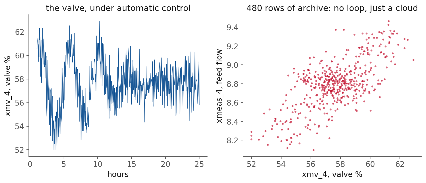
Fig. 16 The same two columns, from 480 logged rows: 24 hours at three-minute sampling. The valve is under automatic control, so it rattles every sample instead of ramping, and the loop is gone. What is left is a cloud with a correlation of +0.69. Note that this run is not quiet operation either. It carries fault 1, a step in the A and C feed ratio, which is a disturbance on the very stream we are identifying. Real archives are like that: the quiet stretches are the ones nobody kept.

Note that the logged data can’t draw the loop at all. That isn’t a flaw in the logged data, and we come back to it at the end of the session, because it’s the most important thing normal operating data does to you.

Let’s be precise about what changed between the two panels of the first figure. Waiting erases the history on purpose. Whatever the loop was doing before, once it settles, the only thing left is the relationship between input and output. That’s why a steady-state calibration needs no column holding the past. Normal operation can’t afford to wait, so the history is still in there.

Continuous-time and discrete-time models

Most models you have previously in your typical engineering classes were probably in continuous time. A mole balance, an energy balance, a rate law, forces acting on a structure: all of them say what is happening at an instant, and they are differential equations.

Definition: continuous-time and discrete-time models

A continuous-time model describes the process at every instant, usually as a differential equation. \(\tau\,dy/dt = -y + Ku\) is one example.

A discrete-time model describes it only at the instants you sampled, as a recipe for the next sample from the ones before it. \(y[t+1] = a\,y[t] + b\,u[t]\) is one.

Your data is discrete. The historian holds one row every three minutes and nothing in between, and a dataframe has rows rather than a continuum. So a possibly model you can fit to a table can be in discrete time, and the question this lecture answers is which columns that table needs and what “shape”.

The continuous model

A vessel or a line with one place to store something (heat, mass, momentum) responds to its input like this:

\[\tau \frac{dy}{dt} = -y + K u\]

in which y is the measurement, u is the valve, and the two constants are what we are after.

Definition: first-order process

A first-order process responds to a step in its input by moving toward a new steady value along an exponential, with no overshoot and no oscillation.

Its time constant \(\tau\) is how long it takes to cover 63 % of the distance. Its steady-state gain \(K\) is how far it eventually goes per unit of input.

Discretizing it: zero-order hold

We want the value at sample \(t+1\) from the value at sample \(t\). To integrate the ODE over that gap we need to know what the valve did in between, and on a real plant the answer is simple: it did nothing. The control system writes one valve position per scan, and the valve sits there until the next action.

Holding the input constant between samples is called zero-order hold (ZOH). Integrate the ODE across one interval \(\Delta t\) on that assumption and two terms come out:

\[y[t+1] = a\,y[t] + b\,u[t], \qquad a = e^{-\Delta t / \tau}, \quad b = K(1 - a)\]

In words: the next flow is most of this flow, plus a bit of the valve.

This is exact, not an approximation, because the valve really is constant between samples.

The discrete model is the feature list

Now read that equation as a specification for a table rather than as physics. It says that to predict row \(t+1\) you need exactly two numbers from row \(t\): the measurement, and the valve.

what the model asks for	the column
\(y[t]\)	the previous measurement, xmeas_4_prev
\(u[t]\)	the valve at that row, xmv_4

That is where the features come from. They are not a guess, and they are not a list of everything in the file. The discretized model names them.

This is the reason the session is about features rather than about fitting. Pick the model structure and the feature table follows; get the table wrong and no fitting routine can repair it.

The two-term model also has a name: an ARX model (autoregressive with exogenous input), specifically ARX(1,1). One lag of the output, one of the input.

Getting the physics back

a and b are what a fit returns, and neither means anything to a plant engineer. Both formulas above invert:

\[\tau = \frac{-\Delta t}{\ln a}, \qquad K = \frac{b}{1 - a}\]

So fit two numbers, substitute, and you have minutes and flow per percent of valve. That is the whole trade from the first page, and it costs two lines of algebra.

The lag plot

Before fitting anything, you can see a directly. Hold the valve still and the model reduces to \(y[t+1] = a\,y[t] + \text{constant}\), which is a straight line. So plot y[t] on one axis and y[t+1] on the other, one point per row. That picture is a lag plot, and its slope is a.

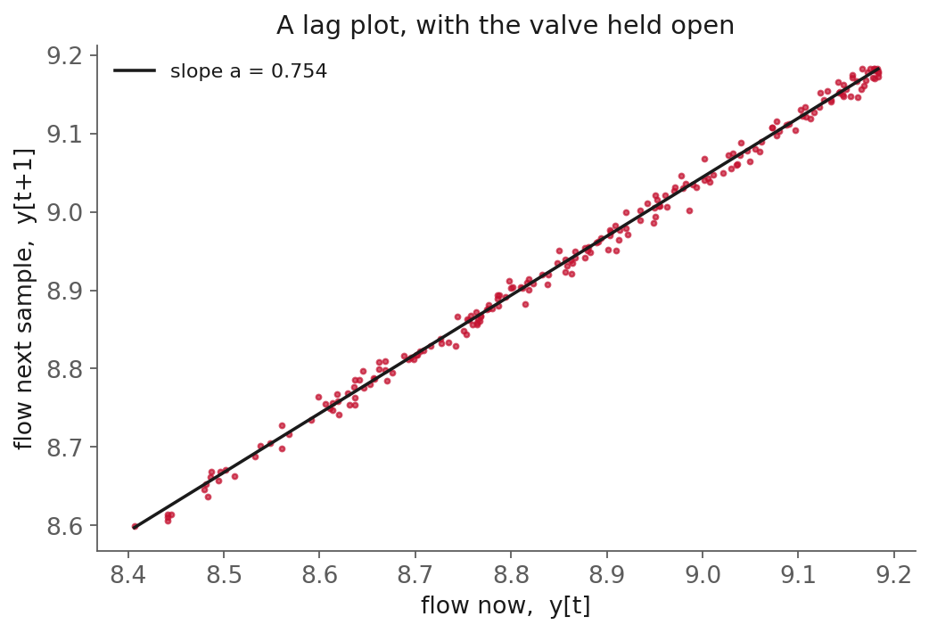
Fig. 17 A lag plot of the same loop with the valve held steady, simulated so the line is clean. The slope is 0.753, and \(\tau = -\Delta t / \ln a\) turns that into 10.6 minutes.

A slope near 1 means each sample is nearly a copy of the last, so the time constant is long. A slope near 0 means the process forgets between samples.

The lag plot works on any series, whatever generated it, and it costs nothing. With the time plot, that is two pictures to draw on a new dataset before fitting anything.

Data leakage

We need a column holding the previous measurement. In Polars (the dataframe library from Lecture 5; pandas spells it the same way) that is shift:

df.with_columns(xmeas_4_prev = pl.col("xmeas_4").shift(1))

shift(1) copies each row’s value down onto the next row. So the row stamped 2:03 PM gets the flow that was measured at 2:00 PM, which is a number you had at 2:03 PM.

shift(-1) copies in the other direction. The row stamped 2:00 PM would get the 2:03 PM reading, which nobody had at 2:00 PM. A model built on that column scores beautifully in testing and is useless in production, because in production the 2:03 PM reading has not happened yet.

One character, and the difference between a working model and a worthless one.

Definition: data leakage

Data leakage happens when a model is trained on information that would not be available at the time it has to make a prediction.

A credit card fraud example

Another good example of the leakage problem has nothing to do with chemical plants. The example is IBM’s.

You are building a model to flag fraudulent credit card transactions. The training file has the customer, the amount, the location, whether fraud was found, and whether a chargeback was received.

A chargeback is the customer disputing the charge. That happens after somebody has decided the transaction was fraud, sometimes weeks after.

So the model learns a rule that is almost perfectly true in the file: a transaction with a chargeback is fraud. Validation looks excellent. Then it goes live, where there is no chargeback column yet, because the whole point is to catch the fraud before anyone disputes anything. The model has nothing to run on and its real accuracy collapses.

Nothing about the data was wrong. The chargeback column is accurate. It just did not exist yet at the moment the prediction was due.

The same thing in our plant data

Two columns in the Tennessee Eastman file are the chargeback in a “different costume”.

faultNumber. It records what was wrong with the plant during that run. Somebody wrote it down after the fact. Put it in the feature table and the model predicts faults perfectly, because you have handed it the answer. In production there is no faultNumber: that is the thing you are trying to produce.

The slow analysers, xmeas_23 through xmeas_41. These are subtler and much easier to ship by accident. A composition analyser runs on a cycle of 6 or 15 minutes. The historian stamps the result against the sample time and holds it until the next cycle, so the row at 14:00 carries a number the control room did not actually have until 14:15. Use it as a feature for a 14:00 prediction and you are reading a result that had not come back yet. It is exactly the chargeback, and the channel screen below is how you find these columns in a file you did not build.

The general shape, in all three cases: a column that gets filled in after the event you are trying to predict.

Two ways leakage gets in

IBM’s website splits it into two:

1. Target leakage. A column in the row holds information from after the row’s timestamp. The chargeback, faultNumber, the analyser. This is a property of the table, so this is the one we fix today.

2. Train-test contamination. The rows used for training come from after the rows used for testing. Shuffle a time series into a random train/test split and every test row has its own neighbours sitting in the training set, so the reported score describes the sampling rate rather than the model.

The second is a modelling decision rather than a table decision and it needs a held-out score to demonstrate, so it belongs with the sessions that fit and evaluate models. But have the idea for now and the fix: split on time, not at random.

The first row of a run

The first row of any run has no previous value, so shift(1) leaves a null there. Drop it. Don’t fill it with zero, which invents a loop at zero flow and asks the fit to explain a step that never happened. In Polars, drop_nulls() after building the lag columns is the whole fix, and losing one row out of four hundred costs nothing.

Record boundaries and the group key

The file holds 192,000 rows. Those rows are not one long dataset. They’re 400 separate experiments, each run on its own simulated plant. shift(1) doesn’t know that, so applied to the sorted table it hands the first row of one experiment the last reading of the one before. Here is the boundary, on xmeas_4:

fault	run	sample	xmeas_4	shift(1)	.over(run)	.over(fault, run)
1	1	500	8.9419	8.8276	8.8276	8.8276
1	2	21	9.2961	8.9419	null	null

The last row of experiment 1 is fine in every column. The first row of experiment 2 claims a previous reading of 8.9419, which came from a different simulated plant. The fabricated value looks plausible, so nothing catches it. Feed flow really is around 9 in both, nothing raises an error, and the row sits in the training data forever.

Before you can group, you have to say what one run is, and here that takes two columns rather than one. Run 1 of fault 1 and run 1 of fault 4 are different plants that happen to share a run number, so .over("simulationRun") isn’t grouping. It’s grouping by half the key.

That mistake is worse than no grouping at all, because it looks like it worked. The check is to count the nulls, since a correct shift leaves exactly one null per experiment:

what you wrote	nulls	boundaries fixed
shift(1)	1	0 of 399
shift(1).over("simulationRun")	20	19 of 399
shift(1).over("faultNumber", "simulationRun")	400	399 of 399

Whenever a log is a concatenation of runs, batches, campaigns or units, the group travels with the shift, and the group is whatever combination of columns identifies one run. Name it once and reuse it, because everything else in this session needs the same key:

GROUP = ["faultNumber", "simulationRun"]     # what identifies one experiment here

Common data preparation operations

Everything above is about one column. Four more operations, all on the same table, one line each.

The clock and the sampling interval

There are no timestamps in this file at all. There is sample, an integer counter, so the first job is to build the clock:

ts = start + sample * 3 minutes

Then check that the rows really are three minutes apart:

df.select(pl.col("ts").diff().value_counts())

Why bother? Because shift(1) reaches back one row, not three minutes. Those are the same thing only when every row is present. If one row is missing, the lag on the row after the gap quietly reaches back six minutes instead of three, and the time constant you fit from it is wrong.

On a clean dataset the check returns one interval. On one with a dropout it returns two or more.

Missing rows are common, for a reason that surprises people. Many plant data systems store a new value only when the reading moves by more than a set amount, so what is stored is uneven on purpose. Somebody then picked an interval when the file was exported, and the file does not say who picked it or what they picked.

Resampling and fill policy

Once you know rows are missing, put them back so the spacing is even again:

df.upsample("ts", every="3m")

That inserts the missing rows and leaves them empty. Now the real question: do you fill them in?

The answer is different for the two columns, and the difference is physical.

Fill the valve. A control system holds its last commanded position until it writes a new one. So if the valve read 57.6 % before the gap, it really was at 57.6 % during the gap. Carrying that value forward records what happened. This is the same zero-order hold from the derivation, showing up again as a cleaning rule.

Do not fill the flow. Nobody measured it during the gap. Carry the last value forward and you have invented a measurement, which then becomes a row you fit against. Least squares cannot tell an invented number from a measured one.

Either way, add a column marking which rows were filled. A table that cannot say which of its numbers were measured is a table nobody can audit.

Rolling window statistics

pl.col("xmeas_4").rolling_std(window_size=10).over(GROUP)

A lag column carries one earlier value. A rolling window statistic carries a summary of many, and on process data those summaries have names you already use. Rolling standard deviation over a control loop is the standard screen for a sticking valve or a transmitter that’s started chattering. Rolling min and max find a channel sitting at its range limit (saturated, or pegged).

The window length is the decision. Longer than your lag depth and it adds something the lag columns don’t carry, namely how agitated the channel has been. Shorter, and it mostly re-describes columns you already have, which leaves lstsq picking one of many equally good answers without telling you.

Note the .over(GROUP), with the same GROUP the shift used. Rolling forgets a run boundary exactly the way shift does.

Channel screening

Ask what fraction of each channel’s rows are identical to the row before:

run.select(pl.col("^xmeas.*$").diff().eq(0).mean())

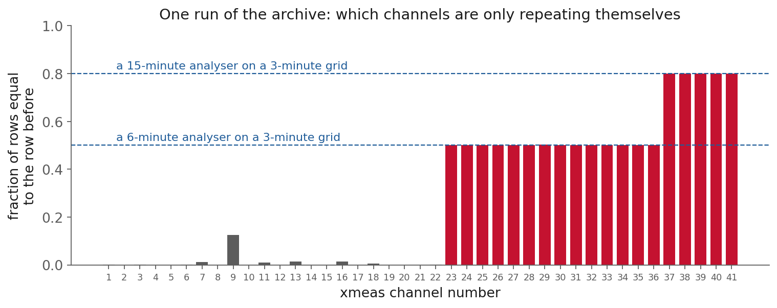
Fig. 18 One run of the logged data, all 41 measured channels. Nineteen of them repeat their previous value on half their rows or more, and they land on two exact plateaus.

Nineteen of the 41 channels come back flat on half their rows or more, at exactly 0.500 and exactly 0.800. Those aren’t quiet sensors. They’re composition analysers running on their own cycle, with the historian holding the last result in between, which is the zero-order hold again. Downs and Vogel give those cycles as 0.1 h for the feed and purge analysers and 0.25 h for the product analyser, so 6 and 15 minutes. On a 3-minute grid that’s exactly one repeat in two and four repeats in five. One line of code recovered the instrument from the data!

A lag feature on a channel like that is a copy of a column you already have.

Sampling interval against time constant

Compare the sampling interval to the time constant you expect. You want several samples inside one time constant, because that’s what it takes for consecutive rows to differ by more than the sensor noise. This loop gives about three and a half, with three-minute samples and a ten-and-a-half-minute time constant.

Sampling that fast has a consequence: consecutive rows barely differ. Guess that nothing changes between one row and the next on reactor pressure and you are wrong by only 9 % of that channel’s spread. Any model of a fast-sampled channel is competing against that. So a fit can look excellent and still be worthless.

Multiple lags and the regression vector

One lag is where you start, not a rule. A loop with two storage terms, or a pipe with transport delay, needs more of its own past before the model can follow it. The general form just keeps going:

\[y[t+1] = a_1 y[t] + a_2 y[t-1] + \dots + b_1 u[t] + b_2 u[t-1] + \dots\]

Nothing about the method changes. Collect the values on the right-hand side into one row vector, which system identification calls the regression vector \(\varphi(t)\):

\[\varphi(t) = [\,y[t],\; y[t-1],\; \dots,\; u[t],\; u[t-1],\; \dots\,]\]

Stack one such row per sample and you have the design matrix \(\Phi\) (the regressor matrix). Collect the coefficients into \(\theta\), and the whole model is one matrix equation:

\[y = \Phi\,\theta\]

lstsq solves that for \(\theta\) whatever the width of \(\Phi\). In Polars, widening the table is the same expression with a different argument:

df.with_columns([
    pl.col("xmeas_4").shift(k).over(GROUP).alias(f"xmeas_4_lag{k}") for k in (1, 2, 3)
])

So how many lags? That question is nontrivial, and we will talk about it in the next lectures.

Lags of a smooth signal are nearly copies of each other. Measured on one run: xmeas_4 correlates with its own first lag at 0.927. On reactor pressure, a slower channel, it is 0.996. So the columns of \(\Phi\) are close to linearly dependent, and least squares is free to trade one nearly-identical column against another.

What that does is measurable. Fitting one lag on this loop gives y[t] a coefficient of 0.753. Fitting three gives it 0.417, with the difference reappearing on y[t-1] and y[t-2], which together sum to about the same number. The memory got spread across the columns.

Note what that costs. With one lag the coefficient is the time constant. With three, no single coefficient converts to anything, so you traded a number you could check against the plant for a slightly better fit.

And every lag you add costs a row at the head of every run, since a table with three lags has no complete row until the fourth sample.

Least squares and the conversion to physics

Finding a and b is one call. Stack the current measurement and the current valve position into a two-column matrix, with the next measurement on the right-hand side, and ask numpy.linalg.lstsq for the least squares solution.

Subtract the mean from each column first. In process control this is working in deviation variables, and here it’s not optional: xmeas_4 sits at 8.79 and xmv_4 at 57.6, so both columns are almost entirely offset. A model with no constant term would spend both coefficients explaining that offset and get a badly wrong.

On one run of the plant data the solve returns a = 0.7529 and b = 0.0322. Converted, that is tau = 10.6 min and K = 0.1304 kscmh per percent of valve. The design matrix has rank 2, meaning its two columns carry genuinely different information.

The output is minutes and kscmh per percent of valve (xmeas_4 is a flow in thousand standard cubic metres per hour). A plant engineer who knows that line can tell you whether ten and a half minutes is credible for it. Nobody can tell you whether an R-squared is credible.

Sensitivity of the time constant to a

The time constant comes out of a logarithm of a number squeezed between 0 and 1, so the conversion amplifies whatever error a carries. How much depends entirely on where a sits.

fitted a	tau	a raised by 1 %	tau
0.7529	10.6 min	0.7604	11.0 min
0.99	298 min	0.9999	30,000 min

At the bottom of the range a 1 % error costs you 3 %. Near 1 the same 1 % error takes a five-hour time constant to three weeks. Two practical consequences. Report a fitted time constant to two significant figures unless you have a reason for more. And treat a fitted a above about 0.99 as a warning rather than a result.

That second one bites on this plant. Many logged channels come back with a near 0.99, which converts to time constants of hours. Three-minute samples are far too close together for a loop that takes hours, so consecutive rows are near-copies, a is pushed toward 1, and the answer reflects the sampling rate and the noise more than the process. Converting to minutes is what catches it. Reported as a score, those channels would have looked excellent, because predicting that a slow channel doesn’t change is easy.

Model structures: ARX, NARX, state space, RNN

You built the smallest member of a large family. The same recurrence runs through all of it.

In process control, ARX(1,1) is the discrete form of the first-order lag you already use. Add dead time and it is FOPDT, the model most PID tuning rules are written against. Widen it to ARX(\(n_a\), \(n_b\)) and you have the workhorse structure of linear system identification.

Make it nonlinear and it becomes NARX: same regression vector, but the function applied to it is no longer a weighted sum. Fit that function with a polynomial, a Gaussian process or a neural network and the name stays the same.

Write it as a state rather than as a list of past outputs and you get a state-space model:

\[x[t+1] = A\,x[t] + B\,u[t], \qquad y[t] = C\,x[t]\]

Our \(a\) and \(b\) are the one-by-one case, in which the state is just the measurement itself.

Now make the state a vector and the update nonlinear and you have a recurrent neural network. An RNN cell is

\[h[t+1] = \tanh(W h[t] + U u[t] + b)\]

which is the same line of arithmetic: some of where you were, plus some of the input. An LSTM is that with gates deciding how much of \(h[t]\) to keep, which is why its name says memory. What changes across the family is how much state you carry and how nonlinear the update is. What does not change is that the past has to be in the table.

Why this matters for the rest of the course

Every model in that list eats the same feature table you just built. If the past is missing from the table, or if a column leaked, no amount of capacity further down the list repairs it. That is why this session is about the table and not about the model.

Limitations: what the data cannot answer

A dataset can be perfectly clean, correctly shifted and free of leakage, and still refuse to answer the question. In both cases below you get a plausible number instead of an error.

The valve that never moved

Freeze the valve at its average and rerun the identical code, which is what the demo does to stand in for a day when the operator left it alone. The rank of the design matrix drops from 2 to 1, b comes back as 0.0000, and the gain converts to 0.000 against a truth of 0.130. The model says the valve does nothing.

The model is right about this data. The valve did nothing, so nothing in the file says what would have happened if it had. No feature engineering recovers that, and no larger model recovers it either, because the information was never collected.

How much movement is enough? Less than you would think. The test is the rank of the design matrix: a constant input leaves it at rank 1, and a single step is enough to bring it to rank 2 and give a usable fit. Only a genuinely constant input fails. That is why plants run step tests, and why an identification experiment adds a small deliberate wiggle to a valve instead of waiting for one to happen.

The name for this in system identification is persistent excitation: the input has to move enough for the parameters to be recoverable at all.

One practical warning

You have to tell the solver what counts as zero. A constant column is exactly zero only after mean-centering, and at the default tolerance lstsq divides by the leftover rounding dust and returns a gain of nine hundred million. Pass an explicit rcond and it returns 0 instead, which is the honest answer.

Closed-loop identification

The second one is harder, because the numbers look like results. Fit reactor temperature against cooling water flow using a year of ordinary plant history, and the coefficient on cooling water comes back positive. The model says that more cooling water goes with a hotter reactor.

The data is right and the question is wrong. During that year the temperature controller was running. It opened the cooling water valve because the reactor got hot, so in the data every increase in cooling follows an increase in temperature. The regression sees the correlation the controller created and reports it.

You wanted to know what happens to the temperature when you open the valve. That’s the opposite causal direction, and the data has almost no evidence about it, because the controller never let the temperature wander far enough to show you.

This is closed-loop identification, and it’s the normal condition of plant historian data. Any loop in automatic during the logging period has had its cause and effect entangled by the controller, and the tighter the control, the less the data can tell you. Under tight control with no external excitation, fitting that data directly pulls the estimate toward the negative inverse of the controller, not toward the process at all. You identify your own PID tuning.

Look back at the logged data cloud from the start of this session. That’s what it was showing you. The valve rattles because the controller is moving it, and no ramp you can see means no loop you can fit.

What a practitioner should take from this

Before fitting anything to normal operating data, find out whether the loop was in automatic. If it was, expect coefficients with the wrong sign, and don’t repair them by removing terms until the signs look right. Two fixes work, and both are experiments. Move the setpoint, so the controller is forced to drive the input over a range while the closed loop keeps the plant safe. Or add a small deliberate excitation to the manipulated variable, large enough to see above the noise and small enough that operations will agree to it. If neither is available, say what the data can and cannot support rather than reporting a coefficient you don’t believe.

In-class demo

The notebook is l07-timeseries.ipynb, in Polars and numpy, and it is deliberately short. It does four things on one run of the feed loop.

1. Load the data and build the clock. The file ships a counter, not timestamps.

2. Build the regressor matrix, twice. Once with one past flow and one past valve position, then again with three and two. Both are printed as tables before anything is fitted, because seeing \(\varphi(t)\) laid out with its columns labelled is the thing prose cannot do.

3. Solve with lstsq and convert. One lag returns a = 0.7529 and b = 0.0322, which is 10.6 minutes and a gain of 0.1304.

4. Freeze the valve and refit. The gain comes back as zero.

Two results are worth watching for, because neither is obvious from the notes.

The deeper model does not blow up, but it does something quieter. The first coefficient drops from 0.753 to 0.417 and the difference reappears on y[t-1] and y[t-2], which sum to roughly the original. Nearly identical columns share the work. And with three lags no single coefficient converts to a time constant any more, so a better fit cost you the number you could check against the plant.

The rest of this session’s material (resampling, fill policy, rolling windows, the channel screen, the group key) stays in these notes rather than in the demo, so the demo can spend its time on the one idea that needs to be seen rather than read.

Summary

A dynamic process needs its own past in the table. The loop picture is why: at one valve position the flow is 8.578 going up and 8.997 coming down, so the valve alone can’t tell you which. The missing column is the previous measurement.

Building that column is one method call. Getting it right is one question, asked of every column in the table: could this value have been printed at the row’s timestamp? That question covers the direction of the shift, the first row of each run, the group the shift has to respect, and the label column that answers the question you were trying to ask. Before you fit, count the intervals, decide which columns may be filled and which may not, and check which channels are only repeating themselves.

Once the table is built, a two-column least-squares solve returns a and b, and the conversions \(\tau = -\Delta t / \ln a\) and \(K = b / (1-a)\) turn them into a time constant and a gain. Widening the table to more lags changes nothing about the method: the regression vector gets longer and lstsq solves the same equation. On this loop that is 10.7 minutes on the dataset we made and 10.6 on the one the plant made. Check those against what you know about the line: a feed loop at ten minutes is arguable, three hours on a three-minute sampler is not, and a gain of exactly zero means the valve never moved.

What you built is an ARX(1,1) model. Make its update nonlinear and it is a NARX; write it with a vector state and it is a state-space model; make that state update nonlinear and it is a recurrent network. All of them read the same feature table. The table comes first.

Resources

• APMonitor, Auto-Regressive Time Series Model.

• scikit-learn, Lagged features for time series forecasting

• Polars, temporal upsampling and rolling aggregations.

• Tennessee Eastman process simulation data (Rieth et al. 2017).

• Downs and Vogel, A plant-wide industrial process control problem (1993).

• O. Nelles, Nonlinear System Identification: From Classical Approaches to Neural Networks, Fuzzy Models, and Gaussian Processes, 2nd ed. (Springer, 2020). Expanded topic of this session, and parts of the following one on nonlinear system identification and time series data. Process control has been identifying models from plant data this way for over fifty years.

Assignment

No assignment is released today. A4 is released at the next session. This week’s deliverable is the practice module, which is where your participation credit for this session comes from.

Practice module

Practice module for this session.