Lecture 6: Streaming concepts and data validation

Overview

• Session Lecture 6, Week 3

• Arc Data Systems

• Slides Deck for this session

• Practice Practice module for this session

• Demo l06-validation.ipynb, a pandera gate that fails loudly, and a windowed replay of the sensor stream

• Assignment 3, released this session; it uses both halves of this week

Why this matters

The pipeline we built in Lecture 5 was a batch pipeline: a clean sequence of stages over a fixed, finished dataset. That is the right picture most of the time, and it is where every team should start. But two facts about real sensor data sit just outside that picture, and a pipeline that ignores them fails quietly rather than loudly. This session is about both, because they are the two ways a data feed betrays the assumptions a batch job makes.

The first fact is that the data does not stop, and it does not arrive in order. A sensor network is an unbounded stream: there is no last row, only the row that has not arrived yet. Worse, the rows arrive jumbled in time. Take the Intel Berkeley Lab feed we have used since Lecture 3, and watch the readings in the order they actually land rather than after sorting. 79.5% of them arrive out of order, meaning a reading whose timestamp is earlier than one already seen from the same mote. That is not a corrupt file; it is the normal behavior of many motes reporting over a lossy network with buffering and retries. A batch job that assumes rows come in time order, or that the dataset is complete when it runs, is simply wrong about this feed, and no amount of care downstream repairs an assumption broken at the source.

The second fact is that the data is not clean, and nothing announces the dirt. The same feed carries physically impossible values: about 18% of its temperature readings fall outside a generous 0-to-50-degree indoor range, and about 26% come from motes whose battery has drained below the level where the sensor can be trusted. Those are not rare outliers to shrug at; they are hundreds of thousands of rows that will quietly pull an average, train a model on nonsense, or trip an alarm, unless something stops them at the door.

Two disciplines answer these two facts. Streaming is how you compute over data that never stops and arrives late: windowing, event time, and watermarks. Data validation is how you stop bad data before it enters: executable checks that run as a gate and fail loudly. The through-line from earlier in the course is the same one Lecture 1 drew from a spreadsheet that silently dropped rows: the cheapest failure to prevent is the one you refuse to let in, and the way you refuse is a check that runs every time.

Learning objectives

By the end of this session you should be able to:

• Distinguish batch from streaming, and identify when sensor systems require streaming.

• Explain windowing, event vs. processing time, watermarks, and late or out-of-order data.

• Author executable data-quality checks and integrate them as a pipeline gate.

Batch, streaming, and the log

A batch job runs on a schedule over a bounded chunk of data: yesterday’s readings, this run’s export, the file that just landed. It has a beginning and an end, it can be rerun, and it is by far the simplest thing to reason about, which is why Lecture 5 built one and why most engineering teams should start there. A streaming system, by contrast, processes an unbounded input as it arrives, record by record, and never runs out of input. The distinction that matters is not the tool but the shape of the data: bounded data invites batch, unbounded data eventually demands streaming, and the honest middle ground, micro-batch, runs a batch job every few seconds over whatever has accumulated, buying most of the latency of streaming with much of the simplicity of batch.

Streams usually travel through a message broker, a server that sits between the programs that write data and the programs that read it. The writers are called producers: a sensor mote, a plant historian, a web server logging clicks. Each producer sends its records to a named topic, such as temperature. The readers are called consumers, and each one subscribes to the topics it cares about: a dashboard, an archive job, an alarm. Producers and consumers never talk to each other directly, only to the broker, so adding a fourth consumer changes nothing for the sensors and a slow consumer cannot stall a fast one. Apache Kafka is the broker most large streaming systems are built on, and it is the one this section describes.

Underneath most streaming systems is one idea worth understanding even if you never operate one: the log. A log is an append-only sequence of records, and it is the abstraction Apache Kafka is built around. A Kafka topic is split into partitions, and, as the Kafka introduction puts it, “when a new event is published to a topic, it is actually appended to one of the topic’s partitions.” Producers append; consumers read forward at their own pace, each tracking an offset, the position of the next record it will read. The ordering guarantee is precise and worth stating precisely, because people routinely overstate it: Kafka guarantees order within a partition, not across a topic. If you need a mote’s readings in order, they must land in the same partition.

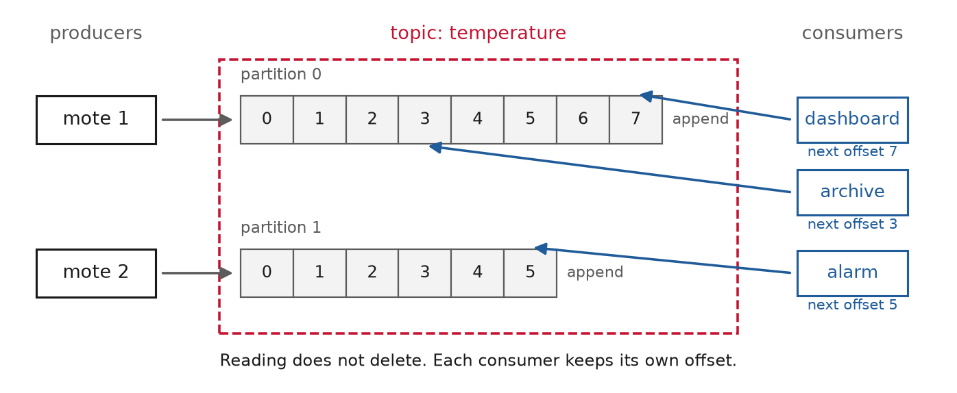
Fig. 11 A topic with two partitions, each an append-only log numbered by offset. Reading a record does not remove it, so each consumer keeps its own position and a slow archive does not hold up the dashboard. A schematic, drawn by figures/make_figures.py.

For the lightest-weight sensor case, the pub/sub protocol you will actually meet on devices is MQTT, “an extremely lightweight publish/subscribe messaging transport” designed for microcontrollers and lossy networks.

Two properties of any such system decide how much you can trust it. The first is delivery semantics. A system is at-most-once if messages can be lost but never redelivered, at-least-once if they are never lost but can be redelivered, and exactly-once if each is processed once and only once. Exactly-once sounds like the obvious choice and is the expensive one, and here is the surprise that trips people: Kafka is at-least-once by default. Exactly-once is not a switch you flip on the cluster; it is opt-in machinery, an idempotent producer plus transactions, or Kafka Streams’ exactly_once_v2 mode, and it constrains how you write your consumers. Assume at-least-once, and design your processing to tolerate a message arriving twice. The second property is backpressure: when a consumer cannot keep up with the rate a producer is pushing, something has to give, and a well-designed pipeline signals upstream to slow down rather than silently dropping data or exhausting memory. The Reactive Streams standard exists precisely so “a fast data source does not overwhelm the stream destination.”

Windows, event time, and watermarks

The question a stream forces on you is one a batch job never has to ask: if the data never ends, what exactly are you aggregating? You cannot take the average of an infinite sequence. The answer is a window, which, in the words of the canonical reference, Akidau and colleagues’ Dataflow Model (VLDB 2015), “slices up a dataset into finite chunks for processing as a group.” Three window shapes cover almost everything. A tumbling window (the paper calls it fixed) has a static size and does not overlap: the average temperature in each clock hour, one number per hour. A sliding window (sometimes hopping) has a size and a shorter step, so windows overlap and the aggregate updates more often: a one-hour average recomputed every fifteen minutes. A session window has no fixed size at all; it groups activity separated by gaps of inactivity, which fits event bursts better than a clock. The paper’s own summary is worth keeping: fixed windows are just the special case of sliding windows where the size equals the step.

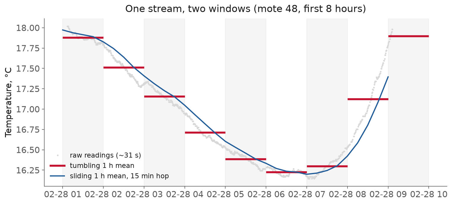
Fig. 12 The same unbounded stream, aggregated two ways. Tumbling one-hour windows (red) produce one non-overlapping mean per hour; a sliding one-hour window stepped every fifteen minutes (blue) overlaps and updates more often. One mote’s temperature over its first eight hours in the Intel Lab feed.

Windows raise a subtler question, and it is the one that separates people who have run a stream from people who have only read about one: which time do you mean? The Dataflow paper draws the line cleanly. Event time is “the time at which the event itself actually occurred,” stamped by the sensor. Processing time is “the time at which an event is observed at any given point during processing.” For a batch over a static file the two barely differ; for a live stream they diverge constantly, because events take a variable, unpredictable time to travel from the sensor to your code. And this is where the 79.5% from the opening returns with teeth. When readings arrive that far out of order, a window defined by processing time, “everything I received between 3:00 and 4:00,” mixes together events that happened at wildly different real times, and the answer is meaningless. You almost always want windows in event time, grouping readings by when they were measured, not when they showed up.

But event-time windows create a problem of their own: if a reading can arrive late, when is it safe to say a window is finished and emit its result? Waiting forever is not an option. The mechanism is a watermark, which the paper defines as “a lower bound (often heuristically established) on event times that have been processed by the pipeline.” A watermark is the system’s best guess that it has now seen all events up to some event time; when the watermark passes the end of a window, the window closes and its result is emitted. A heuristic watermark can be wrong, and a reading can arrive after its window has already closed. That is late data, and a real streaming system needs an explicit policy for it, drop it, or hold windows open long enough to let stragglers in, or re-emit a corrected result when one arrives.

Choosing between those policies is the job of a trigger, which decides when a window emits its result: once, when the watermark passes the end of the window; early, on a timer, if you would rather have a provisional answer sooner than a correct one; or again on each straggler that turns up after the window closed. A window that can emit more than once raises a second question, which is what the later emission means to whoever reads it. That is the accumulation mode. An accumulating window adds the straggler to the result it already sent and re-emits the whole answer, so “the hourly mean is 24.1 degrees” is followed by “correction, 24.3 degrees”; a discarding window sends only the part that is new and leaves the reader to combine the pieces. Both are defensible, and the failure is picking neither, because a dashboard that treats a correction as a fresh reading double-counts every late row.

The Streaming 101 and 102 articles are the readable long form here; 102 is where watermarks and triggers are actually developed, so send yourself there rather than 101 for that part.

Data validation: checks as a gate

Streaming is about when data arrives; validation is about whether it is any good, and it is the more universally useful of the two, because every pipeline, batch or streaming, has data entering it that some upstream process swears is fine. Data validation is the practice of writing down what you expect of the data as executable checks, and running them as a gate: a stage that data must pass before the pipeline will act on it. The checks fall into three kinds, and a good suite has all three. Schema checks assert structure: this column exists, it is a timestamp with a zone, it is a float, it is or is not allowed to be null. Statistical checks assert distributions: the null rate is below some bound, an id is unique, a value’s mean has not drifted off its historical range. Physical-plausibility checks assert what the engineering domain knows: a temperature is inside the instrument’s range, a timestamp does not run backwards, a flow is non-negative. That last category is where engineering data validation earns its keep, because a value can be a perfectly good float and still be physically impossible, exactly the 386-degree readings from Lecture 3.

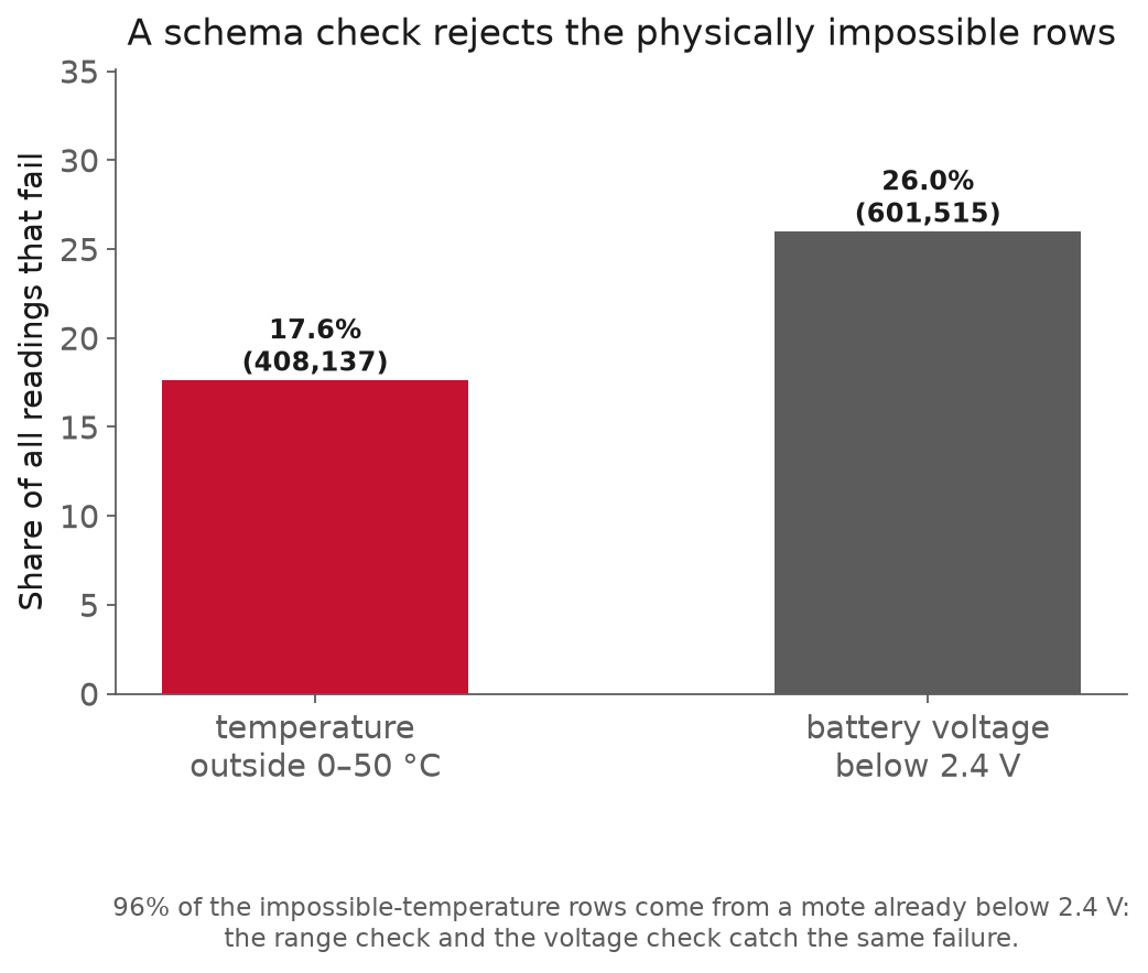
Fig. 13 Two plausibility checks applied to the full Intel Lab feed. A temperature-range check rejects about 18% of readings and a battery-voltage check about 26%, and the two overlap heavily: 96% of the impossible temperatures come from a mote already below 2.4 V. A schema encodes exactly these as executable rules.

The tool that makes this pleasant in Python is pandera, which lets you declare a schema as code. A DataFrameSchema is built from Column objects, each carrying a dtype, a nullability flag, and a list of Checks, where a Check wraps a function that returns a boolean or a boolean series and passes only if every element is true. Built-in checks cover the common cases (Check.in_range, Check.ge, Check.isin, is_monotonic, no_duplicates), and a custom check is just a function, so “temperature between 0 and 50” and “timestamps per mote never decrease” are a few lines each. How it fails is the important part: by default schema.validate(df) raises a SchemaError as soon as one assumption is falsified, and with lazy=True it instead collects every failure and raises a single SchemaErrors with a summary of the offending rows, which is what you want when you are cleaning a genuinely dirty dataset and would rather see all the problems at once than fix them one exception at a time. pandera validates both pandas and Polars frames.

import pandera.pandas as pa

schema = pa.DataFrameSchema({
    "moteid":      pa.Column(int,   pa.Check.isin(range(1, 55))),
    "temperature": pa.Column(float, pa.Check.in_range(0, 50), nullable=True),
    "voltage":     pa.Column(float, pa.Check.ge(2.4),         nullable=True),
})
schema.validate(readings, lazy=True)   # collect every failure, not just the first

Common pitfall

As of pandera v0.24 the recommended import for dataframe validation is import pandera.pandas as pa (with a parallel pandera.polars), and the old top-level import pandera as pa is on its way to deprecation for schemas. The schema code is otherwise identical, so a snippet copied from an older tutorial will still run but may print a deprecation warning. Pin the import to the namespace your version wants, and do not let the warning send students hunting for a bug that is not there.

The heavier alternative is Great Expectations, which is less a library call and more a framework. Its vocabulary, from the GX overview, is worth recognizing: an Expectation is “a verifiable assertion about data,” an Expectation Suite is a collection of them, a Checkpoint runs a suite against data in production, and Data Docs are the human-readable reports it generates. That last piece is the real differentiator: Great Expectations is aimed at teams who want validation results as living documentation a non-engineer can read, at the cost of more setup than a pandera schema. One caution if you reach for it: the workflow changed substantially at the 0.18-to-1.0 boundary (Checkpoints now run “Validation Definitions”), so tie any example to a specific version and do not mix 1.x code with the older docs. For this course, pandera is the default for a pipeline gate and Great Expectations is the tool to know exists when the audience for the results is people rather than code.

Statistical checks are also the seam between validation and monitoring, because a check on a null rate or a monthly mean is the same assertion whether you run it once in a pipeline or forever against production, and a drift you would want an alert for is a check you have already written. A schema also does a second job while it sits there. It is the written-down shape of the data, which makes it a data contract: the agreement between whoever produces a table and whoever consumes it about what the columns are, what they may contain, and what a consumer is entitled to assume. Stated that way it is documentation the next person can build against without reading your loader, and unlike a wiki page it fails the build when it goes stale.

Wherever the checks live, the decision that actually shapes a pipeline is what a failure does. There are three honest options. Block: the pipeline halts and nothing downstream runs, which is right when bad data must never reach a model or a report. Warn: the pipeline logs the problem and continues, which is right for a metric you are monitoring but will not act on immediately. Quarantine: the bad rows are routed aside for inspection while the good ones flow on, which is often the most practical for a large dirty feed where halting on every impossible temperature would stop everything. A check that can only ever pass is untested decoration; the discipline, as with the Lecture 1 demo, is to inject bad data on purpose and prove the gate catches it.

Where streaming and validation push back

Both disciplines in this session are easy to over-apply, and the mature judgment is knowing their limits as well as their uses.

Streaming is a large cost you should defer as long as you can

A batch pipeline is a function you can rerun, inspect, and reason about; a streaming system is a long-lived service with state, watermarks, delivery semantics, and failure modes that only appear under load. The exactly-once machinery is genuinely hard, watermarks are heuristics that will sometimes be wrong, and late data forces a policy decision with no free answer. Most engineering questions, a daily report, a model retrained weekly, an analysis of last month, are batch questions wearing a streaming costume, and the right move is to start with scheduled batch or micro-batch and adopt true streaming only when a real latency requirement forces it. Reaching for Kafka because the data “is a stream” when a nightly job would do is how teams acquire an operational burden they did not need.

A window in event time is only as good as your timestamps

Everything in the windowing section rested on trusting the event-time stamp on each reading. Clock drift is the failure mode: if a sensor’s clock is wrong, or drifts, or resets on a power cycle, then event-time windows group readings by a lie, and no watermark saves you. This is the point where streaming and validation meet: the monotonic-timestamp check from the validation section is not bookkeeping, it is what lets you trust the event times that windowing depends on. Garbage timestamps make sophisticated windowing produce confident nonsense.

Validation confirms plausibility, not correctness

This is the limit worth carrying furthest, and it echoes Lecture 2 exactly: a value that passes every check can still be wrong. A temperature of 24 degrees is inside the plausible range whether or not it is the temperature that actually occurred; a check confirms the reading is possible, not that it is true. Validation catches the impossible and the malformed, which is a large and worthwhile class of error, and it is powerless against a sensor that is miscalibrated but reading plausibly, or a units error that lands inside the allowed range. Do not let a green validation dashboard become the same false comfort that a passing test suite or a reproducible result can be.

A schema is a maintenance burden, and a brittle one fails both ways

Every expectation you encode is a rule someone must maintain as the data legitimately evolves. Set the checks too tight and they cry wolf on every normal fluctuation until the team learns to ignore them, which is worse than no check at all. Set them too loose and they pass the very data they were meant to catch. And a validation suite only ever tests the expectations you thought to write; the failure mode nobody anticipated sails straight through. Validation raises the floor on data quality; it does not cap the ceiling on data problems.

What a practitioner should take from this

Put a validation gate at every boundary where data enters your control, and make failures do something you chose on purpose, block, warn, or quarantine, rather than defaulting to “log and hope.” Write physical-plausibility checks, not just type checks, because engineering data fails in ways a type system cannot see. Treat streaming as a serious commitment to defer: reach for scheduled batch or micro-batch first, and adopt event-time windowing with watermarks only when latency genuinely demands it, remembering that a window is only as trustworthy as the timestamps under it. And hold onto the humbling half of validation: it proves data is plausible, never that it is correct.

In-class demo

The demo runs on a live plant. A Tennessee Eastman simulation publishes to an MQTT broker over WebSockets, and the notebook subscribes to it, collects about three minutes of telemetry, and works on whatever arrived. The figures above come from the Intel Lab replay, where the answers are already known; the demo uses a feed nobody has cleaned, whose numbers come out different every time we run it.

We start with the plant itself, because a reading whose meaning you do not know is a reading you cannot validate: the flowsheet, the 53 tags, and the three gas chromatographs whose readings are stale by a known amount. Then the collector, which writes down exactly what arrived and does nothing else to it. Then the retained birth message, which is the data contract for this feed, and which the validation schema is generated from rather than typed out a second time. Decoding the nested JSON gives one row per reading and three timestamps on each row: when the instrument took it, when the historian published it, and when our machine saw it.

The gate is two schemas, for two different questions. One asks whether the publisher kept its promises, meaning tags from the contract, statuses from the OPC UA set, values inside the physical range for their declared unit, and nothing published before it was measured. The other asks whether the data is fit to average, meaning a real value, a Good status, and one row per tag per reading. The first usually passes and the second always fails, and the failures are the three that recur on any instrument feed: a status code saying the device does not trust its own number, a held analyser value republished on a timer so that a naive count of product composition measurements comes out about five times too high, and readings that arrive after the window they belong to has closed.

The last third is the windowed aggregate. We measure each tag’s staleness and check it against what the contract predicted, and sweep a watermark allowance from zero to three plant hours to price the choice between waiting and dropping. Then we pivot the long table to the wide one an analysis actually wants, one row per sample instant and one column per tag, which is where the missing data finally becomes visible: the 53 tags are not sampled on a common grid, so about a fifth of the table comes out empty, almost all of it in the analyser columns, and a forward fill writes that fifth. We keep the mask of which cells we filled, because a table that cannot say which of its numbers were measured is a table nobody can audit. We finish by computing the same thirty-minute tumbling average twice, once bucketed by event time and once by publish time. Some publish-time windows come out empty, which is a gap on a dashboard for a stretch when the plant was running normally, and the rest are wrong by an amount worth comparing against the tag’s own standard deviation. The runnable notebook is l06-validation.ipynb.

Summary

Real sensor data breaks two assumptions a batch pipeline quietly makes: that the data is finished, and that it is clean. Streaming answers the first. Unbounded, out-of-order data is aggregated with windows, tumbling, sliding, or session, computed in event time rather than processing time, and closed by watermarks that are explicit, heuristic guesses about when late data has stopped arriving. The Intel Lab feed, 79.5% out of order, is why event time and watermarks exist rather than being academic. Validation answers the second. Executable checks, schema, statistical, and physical-plausibility, run as a gate that fails loudly, encoded cleanly with pandera or, for team-readable reports, Great Expectations, and wired to block, warn, or quarantine on failure. On the same feed, a schema rejects about 18% of readings on temperature and 26% on voltage, and the two catch the same dying-battery failure. The honest limits matter as much as the uses: streaming is a cost to defer until latency demands it, and validation proves data plausible, never correct.

Resources

• pandera: DataFrame schemas. Columns, dtypes, and nullability; the shape of a schema-as-code.

• pandera: Checks and lazy validation. Built-in and custom checks, and the difference between SchemaError (fail fast) and SchemaErrors (collect all).

• Great Expectations overview. Expectations, suites, checkpoints, and Data Docs; the heavier, team-readable alternative.

• Akidau et al., The Dataflow Model (VLDB 2015). The canonical treatment of event time, windowing, and watermarks; open access.

• Streaming 101 and Streaming 102. The readable long form; 102 is where watermarks and triggers are developed.

• Apache Flink: Windows. Crisp operational definitions of tumbling, sliding, and session windows, and of late data.

• Apache Kafka: Introduction and delivery semantics. The log abstraction, per-partition ordering, offsets, and at-least-once vs exactly-once.

• MQTT. The lightweight publish/subscribe protocol for internet of things (IoT) and sensor telemetry.

• Reactive Streams. Backpressure as a standard: not overwhelming a slow consumer.

• Intel Lab Data. The streaming/validation feed, carried from Lecture 3, replayed by timestamp. Served over plain HTTP.

• UCI SECOM. A wide, dirty semiconductor feature matrix: about 1,500 runs, roughly 590 process measurements, heavy missingness, a natural target to practise a validation suite on once you have written one here.

• Kleppmann, Designing Data-Intensive Applications, Ch. 11 (“Stream Processing”). The clearest single treatment of logs, streams, and their relationship to batch.

Assignment

Assignment 3, “A plant stream, collected and made trustworthy,” is released this session and is due roughly one week later. You collect at least ten minutes of a live chemical-plant simulation published over MQTT, then build a pipeline that makes what arrived worth computing on. It draws on both halves of this week: Lecture 5’s small, restartable stages and its Polars idioms, and this session’s event time, watermarks, and validation as a gate. With both sessions now covered, you can do the whole assignment. This is a pointer, not the rubric.

Practice module

Practice module for this session, about ten minutes of questions drawn from this session’s notes, slides and demo. It runs entirely in your browser, the questions are selected from your Andrew ID, and it ends by producing a PDF you upload for participation credit.