Lecture 10: The machine learning workflow III, classification, experiment tracking and hyperparameter search

At a glance

• Session Lecture 10, Week 5

• Arc Machine learning and deep learning

• Slides Deck for this session

• Practice Practice module for this session

• Demo l10-classification.ipynb, a fault classifier for the plant; l10-tracking-search.ipynb, a hyperparameter search with Optuna, recorded in MLflow

• Tools scikit-learn for the classifiers, Optuna for the search, MLflow for the record

Why this matters

A chemical plant runs normally almost all the time. A “detector” that always answers “normal” is right 85.4% of the time on the plant data of this session, and it never catches a single fault. Accuracy alone cannot tell that detector from a useful one. This session gives you the tools that can: the confusion matrix, precision and recall.

The second half answers the question Lecture 9 ended on: how do you choose the hyperparameters (the tree depth, the number of hidden units) without guessing? You let a search try them for you, and you keep a record of every try.

Learning objectives

By the end of this session you should be able to:

• Explain what a classifier predicts (a class, from a probability and a threshold), and read a logistic regression’s decision boundary on one plant signal.

• Say what each of the four model families minimizes when it classifies.

• Understand a confusion matrix, and the concepts of accuracy, precision and recall from it.

• Move the decision threshold to trade missed faults against false alarms.

• Explain why a classifier can miss faults it was never trained on.

• Run a hyperparameter search with Optuna, record every trial in MLflow, and register the best model.

Classification

• Regression (Lecture 9) predicts a number: a pressure, a viscosity, a strength.

• Classification predicts a category: normal or faulty, pass or fail, safe or unsafe.

• Most classifiers do it in two steps:

  1. Predict a probability for each class, a number between 0 and 1.

  2. Turn the probability into a class with a threshold: above it, the class is “fault”.

• The four model families of Lecture 9 all have a classification version.

The example: normal or faulty

We use the Tennessee Eastman process (TEP), the simulated chemical plant you have used since Lecture 5. This time we ask a yes-or-no question.

• One sample: one 3-minute snapshot of the plant.

• Features: the 52 channels at that moment (41 measurements and 11 valve positions).

• Target: normal (0) or faulty (1).

• Data: normal runs, and runs where one fault switches on one hour in (Rieth et al., 2017).

• Split by whole run, as in Lectures 8 and 9, so no run is on both sides.

• Training: normal runs 1 to 300, plus runs 1 to 5 of nine faults (1, 2, 4, 5, 6, 7, 8, 12, 13). That is 172,500 samples, 12.5% faulty.

• Test: normal runs 401 to 500, plus runs 11 and 12 of the same nine faults. That is 59,000 samples, 14.6% faulty.

Logistic regression on one channel

Start with one channel and one fault.

• Fault 4 is a step in the temperature of the cooling water entering the reactor.

• The controller reacts by opening the reactor cooling water valve (channel xmv_10) further.

• Normal: the valve sits near 41% open. Fault 4: near 45% open.

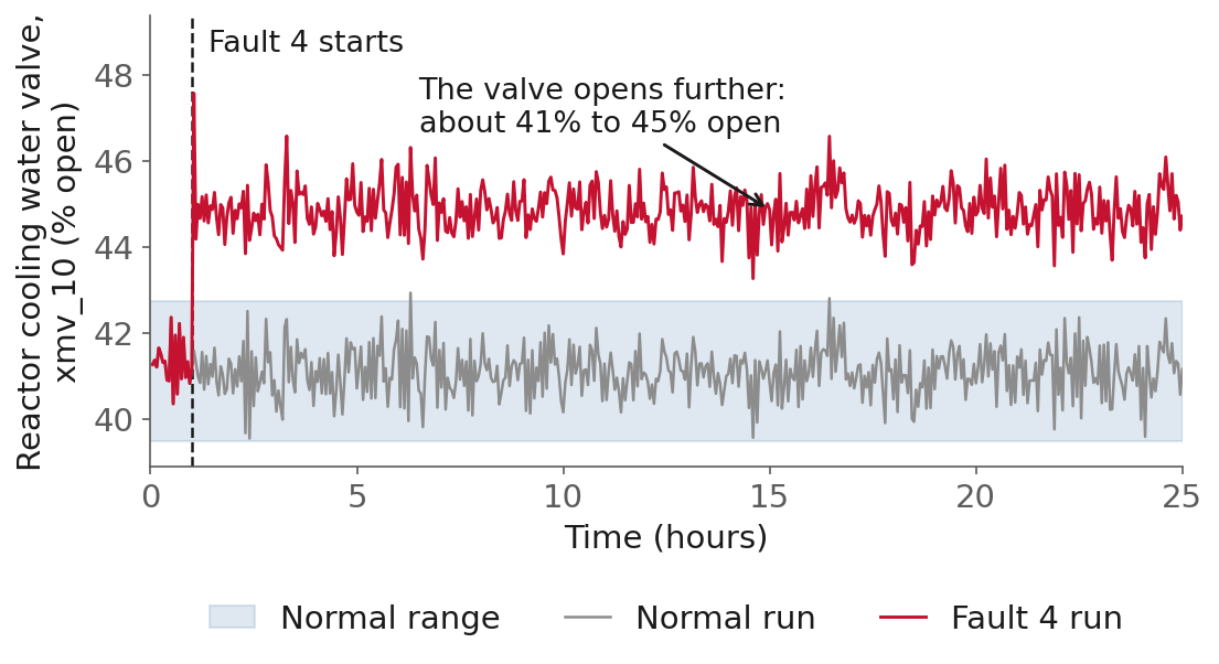
Fig. 56 The valve opening in a normal run and in a fault 4 run. The fault starts at 1 hour.

Definition: logistic regression

Logistic regression turns a weighted sum of the inputs into a probability between 0 and 1.

For one input \(x\) (here, the valve opening):

\[ p(\text{fault} \mid x) = \frac{1}{1 + e^{-(w x + b)}} \]

• \(w x + b\) is a straight-line score, as in linear regression.

• The fraction squashes any score into a probability between 0 and 1.

• The decision boundary is where \(p = 0.5\), that is, where \(w x + b = 0\): \(x = -b / w\).

• Training finds \(w\) and \(b\). Here \(w = 7.24\) per % open and \(b = -314.1\), so the boundary is at \(314.1 / 7.24 = 43.4\%\) open.

• Below 43.4%: normal. Above: fault 4. On the 51,000 test samples this one cut is wrong once (one false alarm).

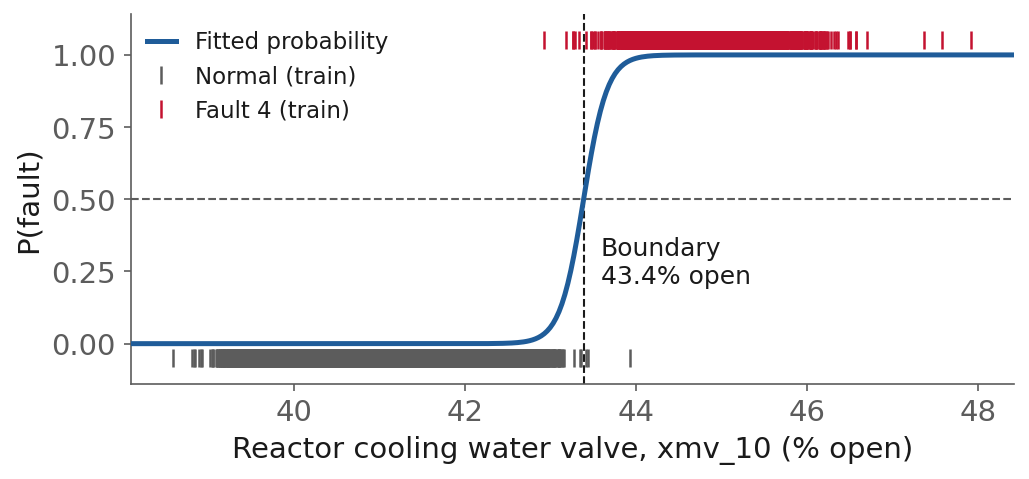
Fig. 57 Logistic regression on the valve opening, normal against fault 4.

When one cut is not enough: fault 14

• Fault 14 makes the same cooling water valve stick.

• The valve swings far open and far closed, but its average stays the same: about 41% open, as in normal runs.

• So the fault samples fall on both sides of the normal range.

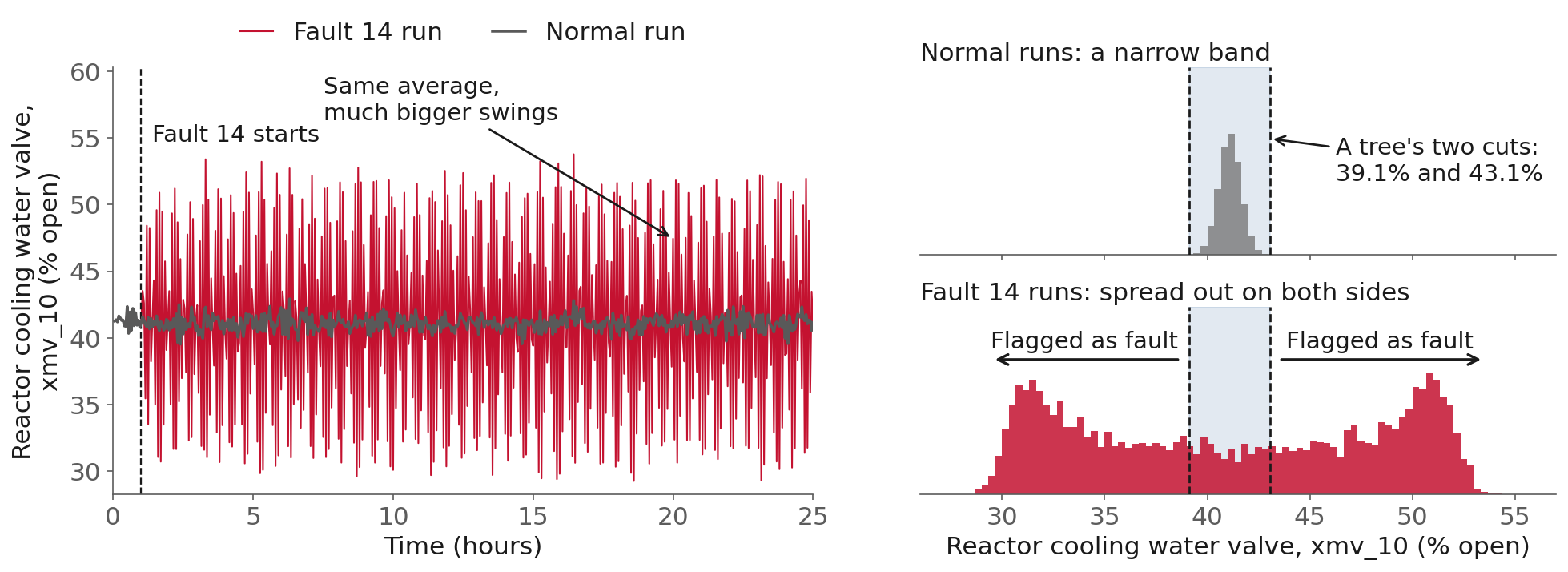
Fig. 58 Fault 14 on the same valve: same average, much bigger swings.

• A logistic regression draws one straight cut. No single cut separates a narrow band from values on both sides of it: it catches 0% of the fault 14 samples.

• A decision tree can make two cuts: “flag anything below 39.13% or above 43.05%”. Two cuts catch 88%; a deeper tree (depth 8) catches 99.7%.

• The shape a model can draw decides what it can catch.

Four model families as classifiers

Each family from Lecture 9 draws a different shape and minimizes a different objective.

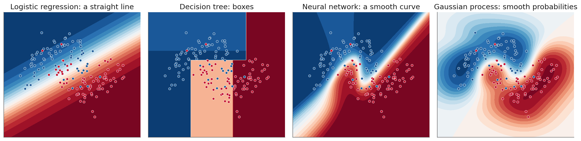
Fig. 59 The shape of the decision boundary each model family can draw, on a small toy dataset.

Logistic regression: a straight line. It minimizes the log loss (also called cross-entropy) over the \(N\) training samples:

\[ L = -\frac{1}{N} \sum_{i=1}^{N} \big[ y_i \log p_i + (1 - y_i) \log (1 - p_i) \big] \]

• \(y_i\) is the true class (0 or 1) and \(p_i\) the predicted probability of class 1.

• The loss is small when the model gives the true class a high probability.

Decision tree: boxes. It splits the inputs with simple questions (is \(x_1 < 43.05\)?), so that each box holds mostly one class. It measures how mixed a box is with the Gini impurity, where \(p_k\) is the fraction of class \(k\) in the box:

\[ G = 1 - \sum_k p_k^2 \]

• \(G = 0\) when a box holds one class only.

• Example: a box with 4 normal samples and 1 faulty one has \(G = 1 - (0.8^2 + 0.2^2) = 0.32\).

• At each step the tree picks the split that lowers \(G\) the most.

Neural network: a smooth curve. The last layer gives one score \(z_j\) per class, and a softmax turns the scores into probabilities:

\[ p_j = \frac{e^{z_j}}{\sum_{k} e^{z_k}} \]

• The probabilities are positive and add up to 1.

• Training minimizes the cross-entropy, \(-\sum_j y_j \log p_j\), which is the log loss above written for any number of classes.

Gaussian process: smooth probabilities. A smooth random function \(f(x)\) (the Gaussian process of Lecture 9) goes through a link function \(\sigma\), often the logistic function above:

\[ p(\text{fault} \mid x) = \sigma\big(f(x)\big) \]

• Near the data the probability is sure (close to 0 or 1). Far from the data it moves back toward 0.5.

• On the plant it is too big to run: its kernel matrix for 172,500 samples would need 238 GB.

Connection to regression. The same families, with a different output and a different loss: a probability instead of a number, and log loss or impurity instead of the squared error.

Measuring a classifier

Why accuracy is not enough

• Accuracy is the fraction of correct predictions.

• Imagine a “detector” that answers normal for every sample, whatever the data says. It is always right on the normal samples and always wrong on the faulty ones.

• On the test samples it scores 85.4% accuracy, because 85.4% of them are normal, and it never catches a fault.

• So we need metrics that tell the two kinds of mistake apart: a missed fault and a false alarm.

The confusion matrix

Definition: confusion matrix

A confusion matrix counts, for every sample, what really happened against what the model said.

We call “fault” the positive class. Each sample lands in one of four boxes:

• True positive (TP): a fault the model caught.

• False negative (FN): a fault the model missed.

• False positive (FP): a false alarm, a normal sample the model called a fault.

• True negative (TN): a normal sample the model left alone.

The numbers below come from one classifier:

• A neural network (one of Lecture 9’s four families) that sees all 52 channels.

• Trained on normal runs 1 to 300 and runs 1 to 5 of the nine training faults.

• Tested on the 59,000 test samples. A sample counts as a fault if it comes from any of the nine faults after the fault starts.

• Threshold 0.5.

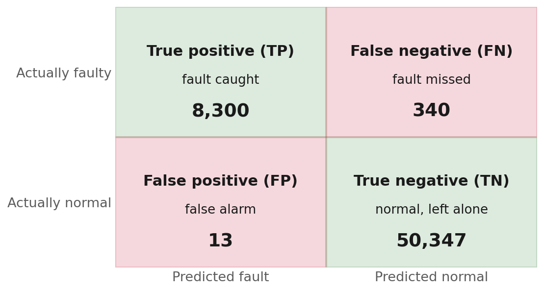
Fig. 60 The confusion matrix of the neural network on the 59,000 test samples.

• The diagonal (TP and TN) is what the model got right.

• The other two boxes are the two kinds of mistakes, and they cost different things: a missed fault can damage the plant; a false alarm wastes an operator’s time.

Accuracy, precision and recall

Definition: precision and recall

Precision is the share of the model’s alarms that were real faults. Recall is the share of the real faults that the model caught.

\[ \text{accuracy} = \frac{TP + TN}{TP + TN + FP + FN} \qquad \text{precision} = \frac{TP}{TP + FP} \qquad \text{recall} = \frac{TP}{TP + FN} \]

On the plant’s test samples:

Classifier	Accuracy	Precision	Recall
Always normal	0.854	0	0
Logistic regression, 52 channels	0.970	0.993	0.803
Decision tree, 52 channels	0.977	0.988	0.855
Neural network, 52 channels	0.994	0.998	0.961

• Always normal never predicts a fault, so TP = 0 and recall is 0. It raises no alarms at all, so precision is 0/0; scikit-learn reports 0.

• The neural network: of its 8,313 alarms, 8,300 were real (precision 0.998); of the 8,640 real fault samples, it caught 8,300 (recall 0.961).

• Accuracy barely separates the last three rows. Recall does.

Moving the threshold

A scikit-learn classifier gives you two things:

• predict(X) returns the class of each sample, using a threshold of 0.5.

• predict_proba(X) returns the probability of each class, so you can choose your own threshold.

Lower the threshold and the model raises more alarms: it catches more faults (recall up) and makes more false alarms (precision down).

Threshold	Faults caught (TP)	False alarms (FP)	Precision	Recall
0.01	8,438	3,664	0.697	0.977
0.10	8,368	265	0.969	0.969
0.50	8,300	13	0.998	0.961
0.90	8,176	0	1.000	0.946
0.99	7,917	0	1.000	0.916

• Threshold ↓: more alarms. Recall ↑ (fewer missed faults), precision ↓ (more false alarms).

• Threshold ↑: fewer alarms. Precision ↑ (fewer false alarms), recall ↓ (more missed faults).

• There is no best threshold in general. Choose it from the cost of a missed fault against the cost of a false alarm.

Faults the classifier never saw

• The network was trained on nine faults. Now test it on eight faults it never saw.

• It learned what those nine faults do to the 52 channels.

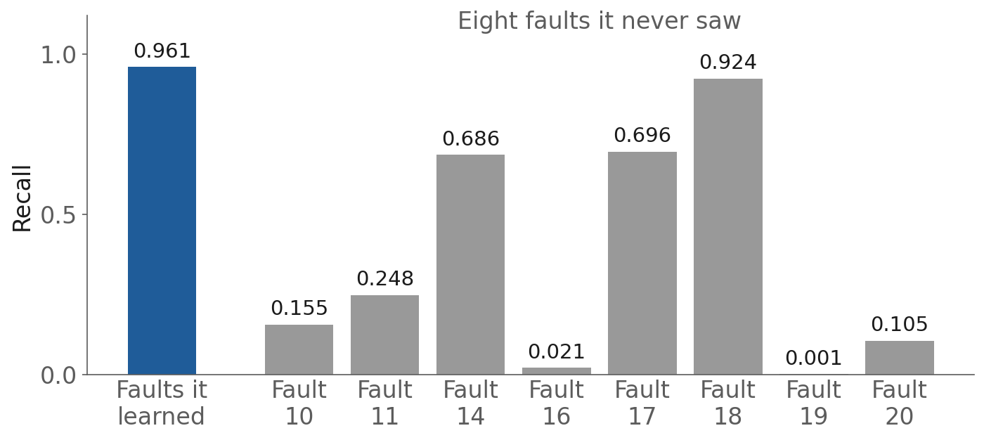
Fig. 61 Recall of the same network on eight faults it was never trained on.

• Each bar is that fault’s recall: the share of its samples the network flagged as a fault (a probability of fault of at least 0.5).

• Recall ranges from 0.924 (fault 18) down to 0.001 (fault 19).

• A new fault is caught when it looks, to the network, like the training faults. Fault 19’s samples look normal to it, so they pass as normal.

• A supervised classifier (Lecture 8) only catches new faults that look like the ones it was trained on.

Tracking and search

Back to Lecture 9’s question

Lecture 9 chose its hyperparameters by hand. For the decision tree on the concrete strength dataset, with the root mean squared error (RMSE) over grouped cross-validation:

• No depth limit: 9.42 MPa.

• The best depth read by eye from the validation curve, depth 9: 9.10 MPa.

Choosing hyperparameters is itself an optimization problem, with training inside it:

\[ \min_{\lambda} \; L_{\text{val}}\big(\theta^*(\lambda)\big) \quad \text{where} \quad \theta^*(\lambda) = \arg\min_{\theta} L_{\text{train}}(\theta; \lambda) \]

• \(\lambda\) are the hyperparameters (the tree depth, the minimum leaf size).

• \(\theta\) are the model’s parameters (the tree’s splits), found by training.

• Every evaluation of the outer problem trains a model. A search needs many of them, and a record of each.

Two tools: Optuna and MLflow

• MLflow (Lectures 1 and 2) records runs: the parameters, the metrics and the model of each one.

• Optuna is an open-source Python library that searches hyperparameters for you (documentation).

  • You write an objective function: it takes a trial’s hyperparameters, trains a model and returns its validation score.

  • Optuna proposes the trials, runs them and keeps the best.

• Together: Optuna runs the search; MLflow records every trial.

Grid search and random search

• Grid search tries every combination on a fixed grid (3 depths times 3 leaf sizes = 9 trials).

• Random search draws each trial’s values at random.

• Usually only a few hyperparameters matter much. With the same number of trials, random search tries more different values of the ones that matter (Bergstra and Bengio, 2012).

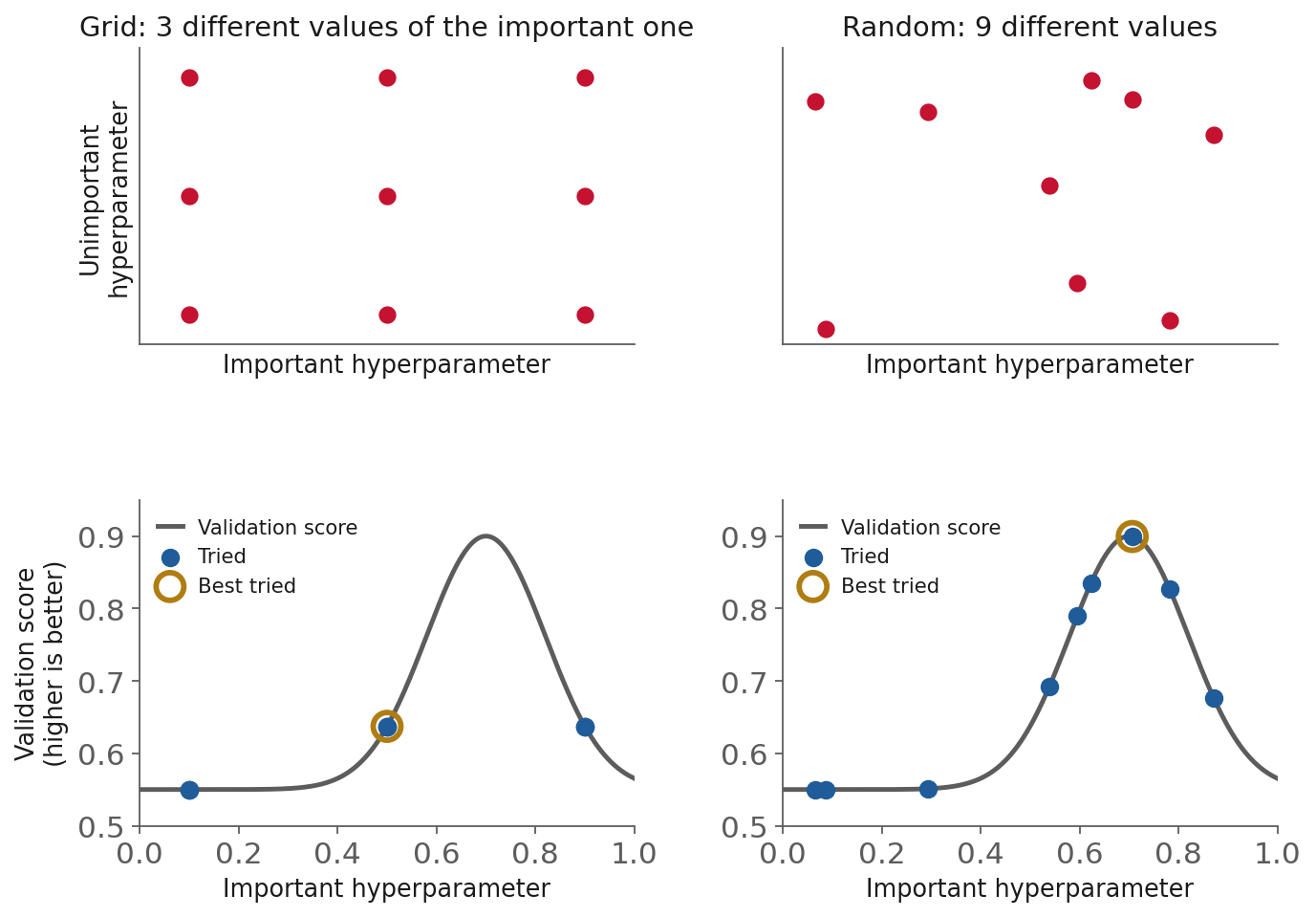
Fig. 62 Nine trials each. The bump is the validation score as a function of the important hyperparameter (made up for the picture): higher is better, and the peak is the best setting.

How to read the figure:

• The square shows the trials: each dot is one pair of values tried.

• The bump below it shows how the score depends on the important hyperparameter. The other one does not change the score.

• Grid search tests only 3 values of the important hyperparameter; random search tests 9, so one of them lands closer to the peak.

• Takeaway: with the same number of trials, random search gets closer to the best setting, because it tries more values of the hyperparameters that matter.

Tree-structured Parzen Estimator (TPE)

Definition: TPE

The Tree-structured Parzen Estimator (TPE) is Optuna’s default search strategy: it uses the trials so far to choose where to try next.

In three steps:

1. Split the trials so far into good ones and bad ones. Optuna calls the best 10% good.

2. Look at where each group’s values of a hyperparameter fall.

3. Try next where good trials are common and bad ones are rare.

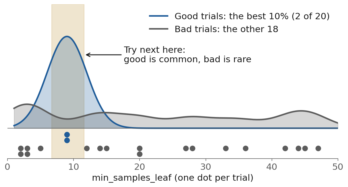
Fig. 63 How TPE picks the next trial, from the first 20 trials of the search below. Each curve is a smoothed histogram of one group’s trials.

• A Parzen estimator is a smoothed histogram, like the two curves in the figure. TPE builds one for the good trials and one for the bad ones.

• Here the two good trials both used a leaf size of 9, and the bad ones are spread out. So TPE tries next near 9: its trials 21 to 26 use leaf sizes from 8 to 13.

• Random search ignores the past; TPE learns from it. In this search, TPE’s first guided trial (trial 11) already scores 8.90 MPa. Random search needs 38 trials to reach 9.00 MPa.

• Why use it: TPE spends the trials where the good results are; random search keeps spending them anywhere. The risk is the opposite one: TPE can settle on one region too early, which is why it starts with 10 random trials.

Optuna inside MLflow

• One MLflow parent run holds the whole search.

• Each Optuna trial is a child run under it: a new max_depth and min_samples_leaf, and the validation RMSE they give. The data, the folds and the model stay the same.

• The best model is refit on all the training rows and registered in the MLflow model registry, with a name and a version anyone can load later.

The demo notebook’s two cells, shortened (SEED = 0; X_tr, y_tr and groups_tr are the training rows, their strengths and their mix labels):

def objective(trial):
    params = dict(
        max_depth=trial.suggest_int('max_depth', 2, 20),
        min_samples_leaf=trial.suggest_int('min_samples_leaf', 1, 50),
    )
    model = DecisionTreeRegressor(
        random_state=SEED,
        **params,
    )
    rmse = -cross_val_score(
        model,
        X_tr,
        y_tr,
        groups=groups_tr,
        cv=GroupKFold(5),
        scoring='neg_root_mean_squared_error',
    ).mean()
    with mlflow.start_run(nested=True):
        mlflow.log_params(params)
        mlflow.log_metric('val_rmse', rmse)
    return rmse

• objective(trial) is called by Optuna once per trial. It returns one number, the score to minimize.

• trial.suggest_int('max_depth', 2, 20) asks Optuna for an integer between 2 and 20.

• cross_val_score(...) scores the tree by five-fold grouped cross-validation, as in Lecture 9: groups=groups_tr keeps each mix in one fold, and scoring= asks for the RMSE (as a negative number, so the minus sign in front makes it positive).

• mlflow.start_run(nested=True) opens a child run inside the parent run. The trial’s settings and its score go into it.

parent = mlflow.start_run(run_name='concrete-tree-search')
study = optuna.create_study(
    direction='minimize',
    sampler=optuna.samplers.TPESampler(seed=SEED),
)
study.optimize(
    objective,
    n_trials=20,
)

• mlflow.start_run(run_name=...) opens the parent run for the whole search.

• direction='minimize' tells Optuna that a lower RMSE is better.

• sampler=TPESampler(seed=SEED) picks TPE, with a fixed seed so the search is repeatable.

• study.optimize(objective, n_trials=20) runs 20 trials.

• The notebook then refits the best settings on all 835 training rows, registers the tree as concrete-tree, and closes the parent run with mlflow.end_run().

The result on the concrete strength dataset

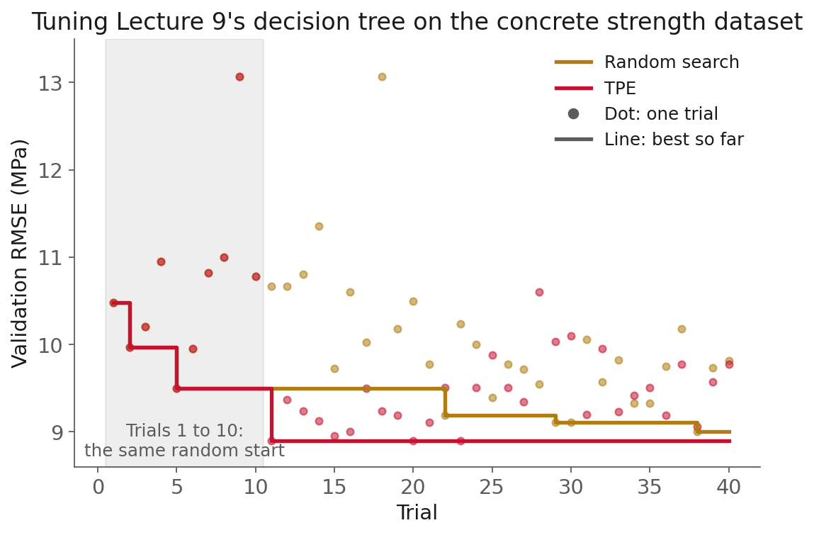
Fig. 64 Each dot is one trial’s validation RMSE; each line is the best RMSE found so far, so it only goes down.

• Best of 40 trials with TPE: 8.90 MPa (max_depth 9, min_samples_leaf 9). With random search: 9.00 MPa (max_depth 16, min_samples_leaf 2).

• Lecture 9’s hand-picked trees scored 9.42 MPa (no depth limit) and 9.10 MPa (depth 9).

• The demo notebook runs the first 20 of those TPE trials and finds the same 8.90 MPa in cross-validation.

• Its winner, registered and loaded back, scores 7.41 MPa on the held-out test mixes. This is the number to report.

• Test once, at the end. The test mixes never took part in the search.

• The test RMSE (7.41) is lower than the validation RMSE (8.90) here. The test set is small (195 rows, 86 mixes), so its score depends on which mixes landed in it.

Limitations and trade-offs

• Precision and recall depend on the threshold. A single number hides the trade-off; report the threshold with them.

• A supervised classifier needs labeled examples of every kind of fault. It can miss a new fault that looks like none of the ones it was shown.

• The four families draw different shapes. A straight-line model cannot catch a fault that widens a signal without moving its average.

• A search is only as good as its objective. Optuna minimizes whatever validation score you give it, so the folds must ask the right question (whole mixes, whole runs).

• Tracking takes discipline. MLflow records what you log; a run with no seed or data version cannot be rebuilt.

In-class demo

• l10-classification.ipynb: the 52-channel fault classifier, its confusion matrix, precision and recall at a few thresholds, and its recall on faults it never saw.

• l10-tracking-search.ipynb: a 20-trial Optuna search for the decision tree on the concrete strength dataset, one MLflow child run per trial, and the winner registered and scored once. Open mlflow ui at the start (section 2) and watch the runs appear.

Summary

• Classification predicts a class: a probability, then a threshold.

• Logistic regression draws one straight cut; a tree can draw several; the shape a model can draw decides what it can catch.

• Accuracy hides the kind of mistake. The confusion matrix counts the four outcomes (TP, FN, FP, TN); precision and recall come from it.

• The threshold trades missed faults against false alarms.

• A classifier only catches new faults that look like the ones it was shown.

• Optuna searches the hyperparameters, TPE uses the past trials to pick the next one, and MLflow records every trial and registers the winner. Test it once.

Resources

• scikit-learn: classification metrics. The confusion matrix, precision, recall and more, with code.

• scikit-learn: Gaussian process classification. The latent function and the link, in more depth.

• Optuna documentation, key features. The objective function, trials and samplers.

• Optuna’s TPESampler. How the default sampler works, with its references.

• MLflow: hyperparameter tuning with child runs. The parent and child run pattern used in this session.

• Bergstra and Bengio (2012), random search. Why random search beats a grid when only a few hyperparameters matter.

• Rieth et al. (2017), the TEP data. The plant runs used here.

Assignment

No assignment is released today.

Practice module

Practice module for this session, for participation credit.