
L11 demo: a gradient by hand, a loop by hand, and three ways to break it#
We build a regression MLP for the UCI Concrete Compressive Strength dataset,
writing the training loop ourselves, and along the way we check that
loss.backward() computes what the chain rule says it should.
Then we break the loop three times on purpose and watch what each failure looks like, because none of them raises an exception.
Requirements. torch, jax, scikit-learn, pandas, matplotlib, and
xlrd. That last one is needed because the canonical copy of this dataset is
still a 1997-vintage .xls and pandas cannot open it otherwise.
Run this first on Colab#
Colab starts from its own preinstalled environment rather than this course’s uv
environment, so run the cell below before anything else. It installs what this
notebook needs and Colab does not already have. Outside Colab it does nothing, so
you can run it or skip it.
# Run this first on Colab. Anywhere else this cell does nothing.
#
# Only genuinely missing packages are installed, so Colab's own versions of
# everything it already ships are left alone.
import importlib.util
import subprocess
import sys

REQUIREMENTS = {
    "jax": "jax",
    "matplotlib": "matplotlib",
    "numpy": "numpy",
    "pandas": "pandas",
    "sklearn": "scikit-learn",
    "torch": "torch",
    "xlrd": "xlrd",
}


def _missing(module):
    try:
        return importlib.util.find_spec(module) is None
    except ModuleNotFoundError:  # the parent package is absent
        return True


if "google.colab" in sys.modules:
    need = sorted({pip for mod, pip in REQUIREMENTS.items() if _missing(mod)})
    if need:
        print("installing:", " ".join(need))
        subprocess.run([sys.executable, "-m", "pip", "install", "-q", *need], check=True)
    print("Colab setup done." if need else "Colab: nothing to install.")
Get the data#
1,030 concrete mixes. Eight inputs (cement, blast-furnace slag, fly ash, water, superplasticizer, coarse and fine aggregate, and age in days) predicting compressive strength in MPa, measured by crushing a cylinder.
That is a real surrogate problem: the target takes 28 days to obtain and destroys the specimen, and the inputs are just the recipe.
import io
import urllib.request
import zipfile
from pathlib import Path

CACHE = Path('.cache')
CACHE.mkdir(exist_ok=True)
LOCAL = CACHE / 'Concrete_Data.xls'
URL = ('https://archive.ics.uci.edu/static/public/165/'
       'concrete+compressive+strength.zip')

if not LOCAL.exists():
    print('downloading', URL)
    with urllib.request.urlopen(URL) as response:
        archive = zipfile.ZipFile(io.BytesIO(response.read()))
    LOCAL.write_bytes(archive.read('Concrete_Data.xls'))

print('cached:', LOCAL, f'({LOCAL.stat().st_size / 1e3:.0f} kB)')
cached: .cache/Concrete_Data.xls (125 kB)
import numpy as np
import pandas as pd

COLUMNS = ['cement', 'slag', 'fly_ash', 'water', 'superplasticizer',
           'coarse_agg', 'fine_agg', 'age_days', 'strength_mpa']
FEATURES = COLUMNS[:8]
MIX = COLUMNS[:7]          # the recipe; age is what varies *within* a mix

concrete = pd.read_excel(LOCAL)          # needs xlrd for .xls
concrete.columns = COLUMNS

print(concrete.shape)
print(concrete.describe().T[['mean', 'std', 'min', 'max']].round(2).to_string())
(1030, 9)
                    mean     std     min     max
cement            281.17  104.51  102.00   540.0
slag               73.90   86.28    0.00   359.4
fly_ash            54.19   64.00    0.00   200.1
water             181.57   21.36  121.75   247.0
superplasticizer    6.20    5.97    0.00    32.2
coarse_agg        972.92   77.75  801.00  1145.0
fine_agg          773.58   80.18  594.00   992.6
age_days           45.66   63.17    1.00   365.0
strength_mpa       35.82   16.71    2.33    82.6
Part 1: tensors, and the dtype that will bite you#
A tensor is a NumPy array that also knows which device it lives on and what was
done to it. It also has a dtype that NumPy would not have chosen, and that is
the first thing to get burned by.
import torch

print('torch', torch.__version__)
print('cuda available:', torch.cuda.is_available(),
      '| mps available:', torch.backends.mps.is_available())

# The trap. NumPy defaults to float64; PyTorch defaults to float32.
print()
print('torch.tensor(3.14).dtype             ->', torch.tensor(3.14).dtype)
print('torch.tensor(np.float64(3.14)).dtype ->', torch.tensor(np.float64(3.14)).dtype)
print('torch.tensor(np.array(3.14)).dtype   ->', torch.tensor(np.array(3.14)).dtype)
print()
print('1.234 stored as float32 is', repr(float(torch.tensor(1.234))))
print('which is off by', abs(float(torch.tensor(1.234)) - 1.234))
print('float32 eps =', np.finfo(np.float32).eps)
torch 2.7.1
cuda available: False | mps available: True

torch.tensor(3.14).dtype             -> torch.float32
torch.tensor(np.float64(3.14)).dtype -> torch.float64
torch.tensor(np.array(3.14)).dtype   -> torch.float64

1.234 stored as float32 is 1.2339999675750732
which is off by 3.2424926743601645e-08
float32 eps = 1.1920929e-07
Note the third line especially: a Python float becomes float32, but a NumPy scalar or 0-d array becomes float64. Nothing about the call site tells you which you have.
And the reason this is hard to catch: float32 promotes to float64 on contact, so every dtype downstream of the mistake reports float64 and looks correct.
a32 = torch.tensor(1.0)                      # float32, by accident
b64 = torch.tensor(np.float64(1.0))          # float64, deliberately
print('a32', a32.dtype, '| b64', b64.dtype, '| a32 + b64 ->', (a32 + b64).dtype)
print('the sum reports float64 even though one input had already lost precision')

# The other classic: a silent broadcast.
pred = torch.randn(64, 1)
target = torch.randn(64)
print()
print('pred', tuple(pred.shape), 'target', tuple(target.shape),
      '-> (pred - target)', tuple((pred - target).shape), '  <-- almost never what you meant')
print('fix it with target[:, None]:',
      tuple((pred - target[:, None]).shape))
a32 torch.float32 | b64 torch.float64 | a32 + b64 -> torch.float64
the sum reports float64 even though one input had already lost precision

pred (64, 1) target (64,) -> (pred - target) (64, 64)   <-- almost never what you meant
fix it with target[:, None]: (64, 1)
Part 2: the gradient, four ways#
Take a network small enough to differentiate by hand: one hidden layer, tanh,
a scalar output, squared-error loss on one example.
The chain rule, with each step reusing the one before it:
That reuse is what reverse-mode autodiff does for you. Now we check it.
from jax import config
config.update('jax_enable_x64', True)     # JAX defaults to float32; we want a fair test
import jax
import jax.numpy as jnp

rng = np.random.default_rng(0)
D, H = 4, 3
W = rng.normal(size=(H, D))
b = rng.normal(size=H)
v = rng.normal(size=H)
c = np.float64(rng.normal())              # np.float64, NOT a bare rng.normal()
x = rng.normal(size=D)
y = np.float64(1.234)                     # likewise


def forward(W, b, v, c):
    return float((v @ np.tanh(W @ x + b) + c - y) ** 2)


def analytic():
    a = np.tanh(W @ x + b)
    dL_dyhat = 2.0 * (v @ a + c - y)
    dL_dz = (dL_dyhat * v) * (1.0 - a ** 2)
    return {'W': np.outer(dL_dz, x), 'b': dL_dz,
            'v': dL_dyhat * a, 'c': np.array(dL_dyhat)}


reference = analytic()
print('analytic dL/dW =')
print(np.round(reference['W'], 6))
analytic dL/dW =
[[ 1.3075e-02 -1.6120e-03  1.7138e-02 -8.3430e-03]
 [ 3.8470e-02 -4.7430e-03  5.0424e-02 -2.4546e-02]
 [ 4.4800e-04 -5.5000e-05  5.8800e-04 -2.8600e-04]]
# --- PyTorch: build a tape, walk it backwards ---------------------------------
tW = torch.tensor(W, requires_grad=True)
tb = torch.tensor(b, requires_grad=True)
tv = torch.tensor(v, requires_grad=True)
tc = torch.tensor(c, requires_grad=True)

loss = (tv @ torch.tanh(tW @ torch.tensor(x) + tb) + tc - torch.tensor(y)) ** 2
loss.backward()
torch_grad = {'W': tW.grad.numpy(), 'b': tb.grad.numpy(),
              'v': tv.grad.numpy(), 'c': tc.grad.numpy()}

# --- JAX: transform the function -------------------------------------------
def loss_fn(params):
    a = jnp.tanh(params['W'] @ x + params['b'])
    return (params['v'] @ a + params['c'] - y) ** 2


jax_grad = {k: np.asarray(g) for k, g in jax.grad(loss_fn)(
    {'W': jnp.array(W), 'b': jnp.array(b),
     'v': jnp.array(v), 'c': jnp.array(c)}).items()}


def worst(g):
    return max(np.max(np.abs(g[k] - reference[k])) for k in reference)


print(f'PyTorch autograd vs analytic : {worst(torch_grad):.3e}')
print(f'jax.grad         vs analytic : {worst(jax_grad):.3e}')
print(f'PyTorch          vs jax.grad : '
      f'{max(np.max(np.abs(torch_grad[k] - jax_grad[k])) for k in reference):.3e}')
print(f'float64 machine epsilon      : {np.finfo(np.float64).eps:.3e}')
PyTorch autograd vs analytic : 1.735e-18
jax.grad         vs analytic : 4.441e-16
PyTorch          vs jax.grad : 4.441e-16
float64 machine epsilon      : 2.220e-16
All three agree to float64 machine precision. Note what makes that true: c and
y were declared as np.float64. Change either to a bare Python float and
PyTorch’s error jumps to about 7.5e-8, which is float32 epsilon, and it looks
like a difference between the libraries rather than a bug in the setup. Try it.
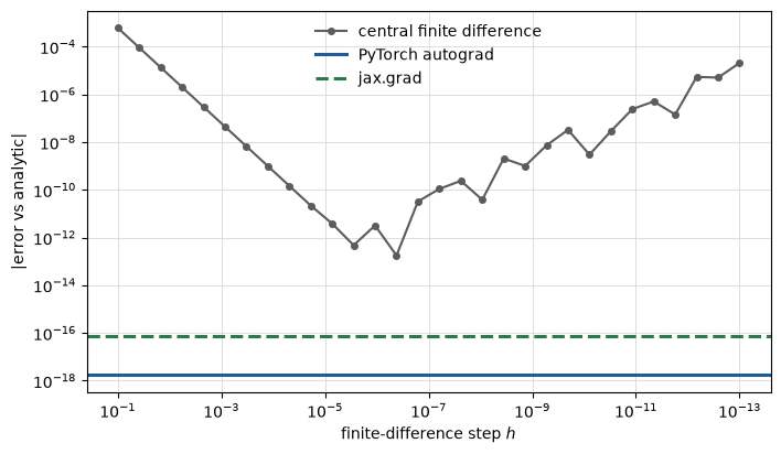
Now the alternative. Finite differences need two forward passes per parameter and are not exact, because the step size trades truncation error against round-off.
import matplotlib.pyplot as plt

steps = np.logspace(-1, -13, 30)
target = reference['W'][0, 0]
errors = []
for h in steps:
    up, down = W.copy(), W.copy()
    up[0, 0] += h
    down[0, 0] -= h
    errors.append(abs((forward(up, b, v, c) - forward(down, b, v, c)) / (2 * h) - target))
errors = np.array(errors)

best = errors.argmin()
print(f'best central difference : {errors[best]:.3e}  at h = {steps[best]:.1e}')
print(f'PyTorch autograd        : {abs(torch_grad["W"][0, 0] - target):.3e}')
n_params = W.size + b.size + v.size + 1
print(f'\nand the cost: {2 * n_params} forward passes for {n_params} parameters,')
print('versus one forward and one backward pass, independent of parameter count.')

fig, ax = plt.subplots(figsize=(8, 4.5))
ax.loglog(steps, np.maximum(errors, 1e-20), 'o-', color='#5c5c5c', ms=4,
          label='central finite difference')
ax.axhline(max(abs(torch_grad['W'][0, 0] - target), 1e-18), color='#1f5c99', lw=2.2,
           label='PyTorch autograd')
ax.axhline(max(abs(jax_grad['W'][0, 0] - target), 1e-18), color='#2b7a4b', lw=2.2, ls='--',
           label='jax.grad')
ax.invert_xaxis()
ax.set_xlabel('finite-difference step $h$')
ax.set_ylabel('|error vs analytic|')
ax.legend(frameon=False, fontsize=10)
ax.grid(True, which='both', color='#d8d8d8', lw=0.6)
ax.set_axisbelow(True)
plt.show()
best central difference : 1.764e-13  at h = 4.2e-07
PyTorch autograd        : 1.735e-18

and the cost: 38 forward passes for 19 parameters,
versus one forward and one backward pass, independent of parameter count.
Part 3: look at the rows before you model them#
Apply L9’s question: are these rows exchangeable? Group them by the seven mix components, ignoring age, and see what happens.
mix_id = concrete.groupby(MIX, sort=False).ngroup().to_numpy()
sizes = pd.Series(mix_id).value_counts()

print(f'{len(concrete)} rows -> {mix_id.max() + 1} distinct mixes')
print(f'mixes tested at more than one age: {(sizes > 1).sum()}')
print(f'   covering {sizes[sizes > 1].sum()} rows '
      f'({sizes[sizes > 1].sum() / len(concrete):.0%} of the dataset)')
print(f'exact duplicate rows (all 9 columns): {concrete.duplicated().sum()}')

biggest = sizes.index[0]
print(f'\nthe most-repeated mix, at {sizes.iloc[0]} different ages:')
print(concrete[mix_id == biggest][['cement', 'water', 'age_days',
                                   'strength_mpa']].to_string(index=False))
1030 rows -> 428 distinct mixes
mixes tested at more than one age: 182
   covering 784 rows (76% of the dataset)
exact duplicate rows (all 9 columns): 25

the most-repeated mix, at 20 different ages:
 cement  water  age_days  strength_mpa
  362.6  164.9         3     35.301171
  362.6  164.9         3     35.301171
  362.6  164.9         3     35.301171
  362.6  164.9         3     35.301171
  362.6  164.9         7     55.895819
  362.6  164.9         7     55.895819
  362.6  164.9         7     55.895819
  362.6  164.9         7     22.897498
  362.6  164.9        28     71.298713
  362.6  164.9        28     71.298713
  362.6  164.9        28     71.298713
  362.6  164.9        28     71.298713
  362.6  164.9        56     77.297154
  362.6  164.9        56     77.297154
  362.6  164.9        56     77.297154
  362.6  164.9        56     77.297154
  362.6  164.9        91     79.296635
  362.6  164.9        91     79.296635
  362.6  164.9        91     79.296635
  362.6  164.9        91     79.296635
Three quarters of the rows share a mix with another row: the same batch of concrete, cured for different lengths of time, recorded as separate rows. A random k-fold puts the same mix on both sides of the split and asks the model to fill in a curing curve it has already seen most of.
We also get a rough handle on the noise floor. A few settings have the same mix at the same age measured twice, which is a repeatability measurement.
dup = concrete[concrete.duplicated(subset=FEATURES, keep=False)]
pairs = [abs(g['strength_mpa'].iloc[0] - g['strength_mpa'].iloc[1])
         for _, g in dup.groupby(FEATURES)
         if len(g) == 2 and g['strength_mpa'].nunique() == 2]

print(f'{len(pairs)} settings measured twice with different results:')
print('  |differences| =', np.round(sorted(pairs), 2))
print(f'  repeatability std = sqrt(mean(d^2)/2) = {np.sqrt(np.mean(np.square(pairs)) / 2):.2f} MPa'
      f'   ({len(pairs)} degrees of freedom)')
print(f'\nfor scale, the target standard deviation is '
      f'{concrete["strength_mpa"].std():.2f} MPa')
print('Treat that as an order of magnitude, not a number: 8 dof is very few.')
8 settings measured twice with different results:
  |differences| = [0.89 1.28 1.48 1.68 1.97 2.86 3.44 6.6 ]
  repeatability std = sqrt(mean(d^2)/2) = 2.16 MPa   (8 degrees of freedom)

for scale, the target standard deviation is 16.71 MPa
Treat that as an order of magnitude, not a number: 8 dof is very few.
Part 4: the training loop, written by hand#
Four objects and five lines. We use a Dataset and DataLoader even though this
table fits in memory, because A6 will need them for anything windowed.
from torch import nn
from torch.utils.data import DataLoader, TensorDataset
from sklearn.model_selection import GroupKFold
from sklearn.preprocessing import StandardScaler

SEED = 0
X = concrete[FEATURES].to_numpy(np.float32)
y = concrete['strength_mpa'].to_numpy(np.float32)

# Hold out whole mixes, not random rows.
folds = list(GroupKFold(5).split(X, y, mix_id))
train_idx, val_idx = folds[0]
print(f'fold 0: {len(train_idx)} train rows, {len(val_idx)} validation rows')
print(f'mixes shared between the two sides: '
      f'{len(set(mix_id[train_idx]) & set(mix_id[val_idx]))}')


def make_mlp(width=64, depth=2, d_in=8):
    layers, d = [], d_in
    for _ in range(depth):
        layers += [nn.Linear(d, width), nn.ReLU()]
        d = width
    return nn.Sequential(*layers, nn.Linear(d, 1))


print(f'\nparameters in a 2x64 MLP: '
      f'{sum(p.numel() for p in make_mlp().parameters()):,}')
fold 0: 824 train rows, 206 validation rows
mixes shared between the two sides: 0

parameters in a 2x64 MLP: 4,801
def train(train_idx, val_idx, *, width=64, depth=2, lr=1e-3, epochs=300, batch=64,
          zero_grad=True, scale=True, device='cpu', seed=SEED, optimizer='adam',
          record=False):
    """A hand-written training loop. `zero_grad` and `scale` can be switched off
    so the failures can be measured instead of described."""
    torch.manual_seed(seed)
    X_tr, X_va = X[train_idx], X[val_idx]
    y_tr, y_va = y[train_idx], y[val_idx]

    if scale:                                   # fit on TRAIN only, as always
        scaler = StandardScaler().fit(X_tr)
        X_tr = scaler.transform(X_tr).astype(np.float32)
        X_va = scaler.transform(X_va).astype(np.float32)
    y_mean, y_std = y_tr.mean(), y_tr.std()

    dev = torch.device(device)
    loader = DataLoader(
        TensorDataset(torch.tensor(X_tr, device=dev),
                      torch.tensor((y_tr - y_mean) / y_std, device=dev)[:, None]),
        batch_size=batch, shuffle=True)
    xv = torch.tensor(X_va, device=dev)
    yv = torch.tensor(y_va, device=dev)[:, None]

    model = make_mlp(width, depth, X_tr.shape[1]).to(dev)
    opt = (torch.optim.Adam(model.parameters(), lr=lr) if optimizer == 'adam'
           else torch.optim.SGD(model.parameters(), lr=lr))
    loss_fn = nn.MSELoss()
    history = []

    for _ in range(epochs):
        model.train()
        for xb, yb in loader:
            loss = loss_fn(model(xb), yb)       # forward
            if zero_grad:
                opt.zero_grad()                 # clear the accumulator
            loss.backward()                     # backward
            opt.step()                          # update
        if record:
            model.eval()
            with torch.no_grad():               # do not build a graph we will not use
                history.append(float(torch.sqrt(torch.mean(
                    (model(xv) * y_std + y_mean - yv) ** 2))))

    model.eval()
    with torch.no_grad():
        rmse = float(torch.sqrt(torch.mean((model(xv) * y_std + y_mean - yv) ** 2)))
    return rmse, history


baseline = float(np.sqrt(np.mean((y[val_idx] - y[train_idx].mean()) ** 2)))
rmse, _ = train(train_idx, val_idx)
print(f'predict the training mean : {baseline:6.2f} MPa')
print(f'the MLP                   : {rmse:6.2f} MPa')
predict the training mean :  17.86 MPa
the MLP                   :   5.94 MPa
Part 5: break it three times#
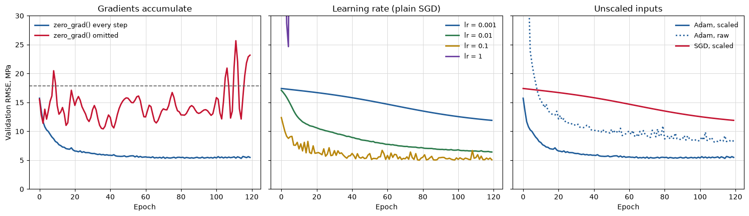
Each of these is a real bug people write. None of them raises.
fig, axes = plt.subplots(1, 3, figsize=(15, 4.4), sharey=True)
RED, BLUE, GREEN, AMBER = '#c41230', '#1f5c99', '#2b7a4b', '#b8860b'
EPOCHS = 120

# --- 1. the missing zero_grad() --------------------------------------------
for flag, colour, label in ((True, BLUE, 'zero_grad() every step'),
                            (False, RED, 'zero_grad() omitted')):
    r, hist = train(train_idx, val_idx, epochs=EPOCHS, zero_grad=flag, record=True)
    axes[0].plot(hist, color=colour, lw=2, label=label)
    print(f'zero_grad={str(flag):5s} -> {r:8.2f} MPa')
axes[0].axhline(baseline, color='#5c5c5c', ls='--', lw=1.2)
axes[0].set_title('Gradients accumulate')
axes[0].set_ylabel('Validation RMSE, MPa')

# --- 2. the learning rate, with plain SGD ----------------------------------
print()
for lr, colour in zip((1e-3, 1e-2, 1e-1, 1.0, 2.0),
                      (BLUE, GREEN, AMBER, '#6b3fa0', RED)):
    r, hist = train(train_idx, val_idx, epochs=EPOCHS, lr=lr, optimizer='sgd',
                    record=True)
    hist = np.asarray(hist)
    if np.isfinite(hist).any():
        axes[1].plot(np.where(np.isfinite(hist), hist, np.nan), color=colour, lw=2,
                     label=f'lr = {lr:g}')
    print(f'SGD lr={lr:<6g} -> {r:14.2f} MPa   '
          f'({int((~np.isfinite(hist)).sum())}/{len(hist)} epochs non-finite)')
axes[1].set_title('Learning rate (plain SGD)')

# --- 3. unscaled inputs, two optimizers ------------------------------------
print()
for opt_name, colour in (('adam', BLUE), ('sgd', RED)):
    for scale, style in ((True, '-'), (False, ':')):
        r, hist = train(train_idx, val_idx, epochs=EPOCHS, scale=scale,
                        optimizer=opt_name, record=True)
        hist = np.asarray(hist)
        if np.isfinite(hist).any() and (hist < 40).any():
            axes[2].plot(np.where(np.isfinite(hist), hist, np.nan), color=colour,
                         lw=2, ls=style,
                         label=f'{"Adam" if opt_name == "adam" else "SGD"}, '
                               f'{"scaled" if scale else "raw"}')
        print(f'{opt_name:4s} scale={str(scale):5s} -> {r:14.2f} MPa')
axes[2].set_title('Unscaled inputs')

for ax in axes:
    ax.set_xlabel('Epoch')
    ax.set_ylim(0, 30)
    ax.legend(frameon=False, fontsize=9.5)
    ax.grid(True, color='#d8d8d8', lw=0.7)
    ax.set_axisbelow(True)
fig.tight_layout()
plt.show()
zero_grad=True -> 5.49 MPa
zero_grad=False -> 23.18 MPa
SGD lr=0.001 -> 11.90 MPa (0/120 epochs non-finite)
SGD lr=0.01 -> 6.42 MPa (0/120 epochs non-finite)
SGD lr=0.1 -> 5.07 MPa (0/120 epochs non-finite)
SGD lr=1 -> 91.02 MPa (0/120 epochs non-finite)
SGD lr=2 -> nan MPa (120/120 epochs non-finite)
adam scale=True -> 5.49 MPa
adam scale=False -> 8.26 MPa
sgd scale=True -> 11.90 MPa
sgd scale=False -> nan MPa
Read the three panels in order.
zero_grad() is the one that should worry you most, because the broken run
scores worse than predicting the mean and its curve oscillates rather than
diverging, so it reads as a tuning problem rather than a bug.
The learning rate fails totally rather than gradually. With SGD, 2.0 gives
nan from the first epoch on every seed tried: there is no partially-diverged
run to inspect. 1.0 sits right on the stability boundary, and whether it blows
up or merely diverges to a few hundred MPa depends on the seed, which is worth
knowing before you conclude that a learning rate is “fine”.
Unscaled inputs behave completely differently depending on the optimizer. SGD diverges. Adam does not, and quietly hands you a model roughly twice as bad as it should be. Adam’s forgiveness is what hides the bug.
Part 6: the accelerator#
Moving to a GPU is two lines. Whether it helps is a measurement, not an assumption.
import time

devices = ['cpu'] + (['mps'] if torch.backends.mps.is_available() else [])
if torch.cuda.is_available():
    devices.append('cuda')
print('available:', devices)

results = {}
for dev in devices:
    best = float('inf')
    for _ in range(3):
        t0 = time.perf_counter()
        rmse, _ = train(train_idx, val_idx, epochs=20, device=dev)
        if dev == 'mps':
            torch.mps.synchronize()
        elif dev == 'cuda':
            torch.cuda.synchronize()
        best = min(best, (time.perf_counter() - t0) / 20)
    results[dev] = (best * 1e3, rmse)
    print(f'{dev:5s}: {best * 1e3:7.2f} ms/epoch   validation RMSE {rmse:.3f} MPa')

if len(results) > 1:
    slowest = max(results, key=lambda d: results[d][0])
    fastest = min(results, key=lambda d: results[d][0])
    print(f'\n{fastest} is {results[slowest][0] / results[fastest][0]:.1f}x faster '
          f'than {slowest} for this model.')
    print('Same architecture, same seed, same answer. The device is a throughput')
    print('choice, and this model is far too small to amortise a kernel launch.')
available: ['cpu', 'mps']
cpu : 3.86 ms/epoch validation RMSE 6.768 MPa
mps  :   21.11 ms/epoch   validation RMSE 6.768 MPa

cpu is 5.5x faster than mps for this model.
Same architecture, same seed, same answer. The device is a throughput
choice, and this model is far too small to amortise a kernel launch.
Part 7: does the net beat the tree?#
Now the comparison the module asks for, on the same folds, under both split schemes. Three seeds here to keep the notebook quick; the figure in the notes uses five and reaches the same conclusion.
from sklearn.ensemble import HistGradientBoostingRegressor
from sklearn.model_selection import KFold

SCHEMES = {
    'GroupKFold by mix (honest)': list(GroupKFold(5).split(X, y, mix_id)),
    'KFold random rows (leaky)': list(KFold(5, shuffle=True, random_state=SEED).split(X)),
}
N_SEEDS = 3
summary = {}

for name, scheme in SCHEMES.items():
    tree_scores, net_scores = [], []
    for seed in range(N_SEEDS):
        for tr, va in scheme:
            tree = HistGradientBoostingRegressor(random_state=seed).fit(X[tr], y[tr])
            tree_scores.append(float(np.sqrt(np.mean((y[va] - tree.predict(X[va])) ** 2))))
            net_scores.append(train(tr, va, seed=seed)[0])
    tree_scores, net_scores = np.array(tree_scores), np.array(net_scores)
    gap = net_scores - tree_scores
    summary[name] = (tree_scores, net_scores, gap)
    print(f'{name}')
    print(f'   gradient boosting {tree_scores.mean():6.3f} +/- {tree_scores.std():.3f}')
    print(f'   MLP (PyTorch)     {net_scores.mean():6.3f} +/- {net_scores.std():.3f}')
    print(f'   MLP minus tree    {gap.mean():+6.3f} +/- {gap.std() / np.sqrt(len(gap)):.3f}'
          f'  (standard error)')
    verdict = ('the tree wins' if gap.mean() > 2 * gap.std() / np.sqrt(len(gap))
               else 'too close to call')
    print(f'   verdict: {verdict}\n')
GroupKFold by mix (honest)
   gradient boosting  6.252 +/- 0.456
   MLP (PyTorch)      6.336 +/- 0.560
   MLP minus tree    +0.084 +/- 0.218  (standard error)
   verdict: too close to call
KFold random rows (leaky)
   gradient boosting  4.440 +/- 0.314
   MLP (PyTorch)      4.973 +/- 0.366
   MLP minus tree    +0.532 +/- 0.110  (standard error)
   verdict: the tree wins
Both models get worse when the leak is closed, which is expected. The question is which gets worse faster, and the answer is the tree: gradient boosting is better at exploiting a near-duplicate row than a small MLP is.
So on this dataset, honestly evaluated, the two tie. Under a random split the tree “wins” by a margin that is entirely an artefact of the split.
That is a narrow claim about one 1,030-row dataset, not a refutation of Grinsztajn et al., who benchmarked 45 datasets and found trees still state of the art on tabular data. The generalisable part is the method: check that a model-family gap is not a split artefact before you explain it with inductive bias.
What to take away#
Autodiff is exact, and finite differences are not. Both frameworks matched the hand-derived gradient to float64 epsilon. The best finite difference, over thirty step sizes, was four orders of magnitude worse and required knowing the right step in advance.
PyTorch accumulates into a mutable .grad, which is why zero_grad() exists.
JAX transforms pure functions and has nothing to zero. Knowing that turns the
rule into a consequence.
Set your dtypes at the boundary. A Python float becomes float32, promotion hides it downstream, and the cost is float32 epsilon on every gradient.
Adam hides scaling bugs; SGD announces them. Neither is better; you just need to know which failure you are looking at.
The GPU is a throughput device. This model is faster on the CPU, and that is the normal case for tabular engineering data.
And run a baseline. A6 asks for a classical comparison on the same split for exactly the reason this notebook demonstrates.