L6 demo: validating a live plant stream

This notebook connects to a running plant, collects a few minutes of its telemetry, and puts that telemetry through the two ideas of this session: a schema used as a gate, and a windowed aggregate computed in event time.

The feed is the same one Assignment A3 collects from, and it is live. Nobody has cleaned it, the numbers are different every time you run this, and some of what arrives is wrong or late. Read the printed output rather than trusting a number written in a markdown cell, because there are none.

Run this first on Colab

Colab starts from its own preinstalled environment rather than this course’s uv environment, so run the cell below before anything else. It installs what this notebook needs and Colab does not already have. Outside Colab it does nothing, so you can run it or skip it.

# Run this first on Colab. Anywhere else this cell does nothing.
#
# Only genuinely missing packages are installed, so Colab's own versions of
# everything it already ships are left alone.
import importlib.util
import subprocess
import sys

REQUIREMENTS = {
    "matplotlib": "matplotlib",
    "paho": "paho-mqtt",
    "pandas": "pandas",
    "pandera.pandas": "pandera",
}


def _missing(module):
    try:
        return importlib.util.find_spec(module) is None
    except ModuleNotFoundError:  # the parent package is absent
        return True


if "google.colab" in sys.modules:
    need = sorted({pip for mod, pip in REQUIREMENTS.items() if _missing(mod)})
    if need:
        print("installing:", " ".join(need))
        subprocess.run([sys.executable, "-m", "pip", "install", "-q", *need], check=True)
    print("Colab setup done." if need else "Colab: nothing to install.")

1. The plant

The Tennessee Eastman process is a chemical plant published by Downs and Vogel in 1993 as a control and monitoring benchmark, and it has been one ever since. Four gaseous reactants (A, C, D, E) plus an inert (B) and a byproduct (F) go in; two liquid products (G and H) come out.

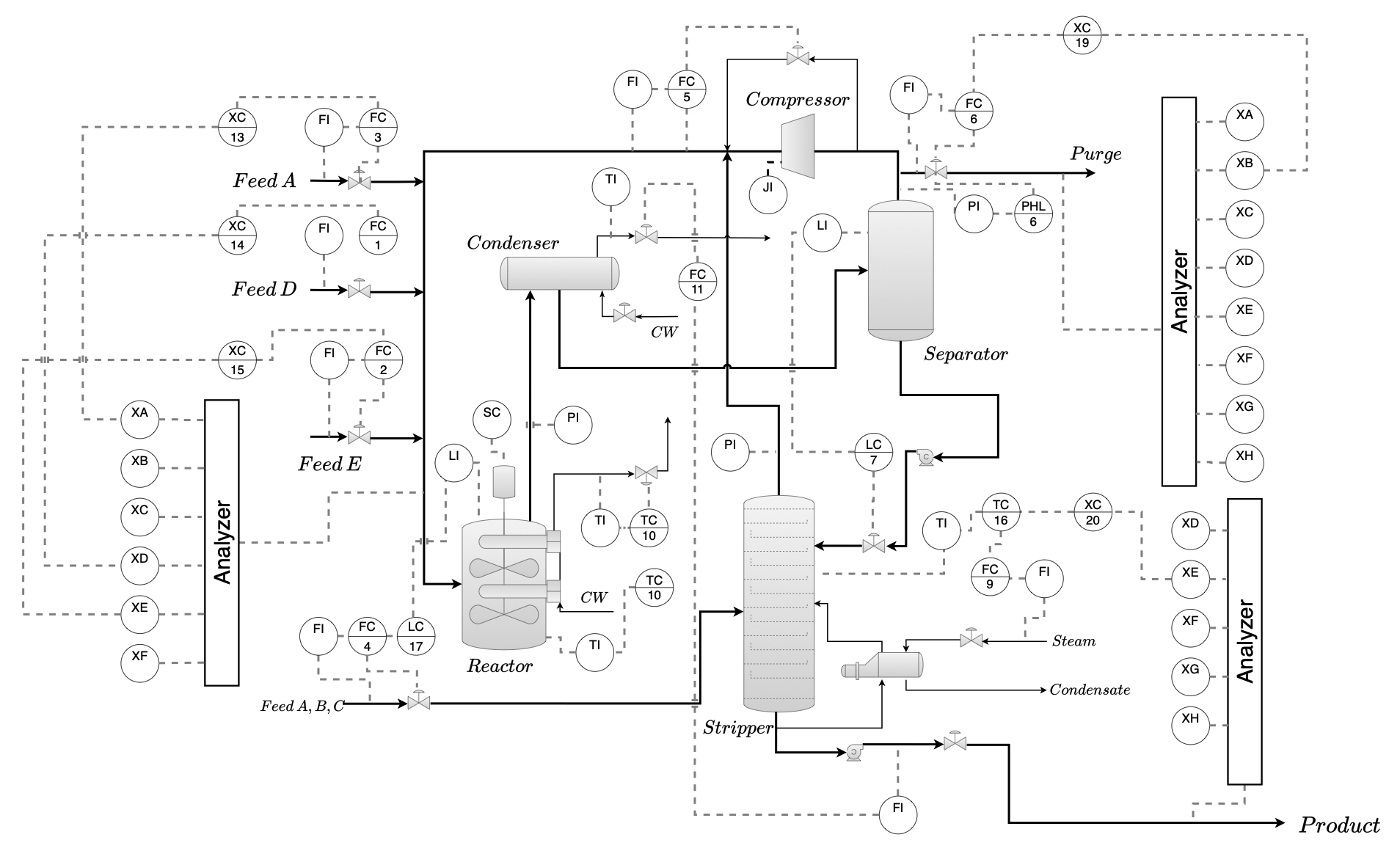
Figure from Lyu, Botcha, Kulkarni, Pagaria, Alves, Sunshine, and Kitchin (2026). You can run the simulator yourself at TEP Studio.

Follow the flowsheet left to right. Feeds A, D and E and a combined A/B/C stream enter a reactor, which is where the reaction happens and which is cooled by a water coil. Its vapour goes to a condenser, then to a separator that splits the condensed liquid from the gas. The gas is recycled through a compressor back to the reactor, with a small purge stream bleeding off so the inert B does not accumulate until the plant chokes. The separator’s liquid drops into a stripper, which boils the light components back out with steam, and what leaves the bottom of the stripper is the product.

Three blocks on the diagram are labelled Analyzer, on the reactor feed, on the purge and on the product. Those are gas chromatographs, and they are the reason this plant is interesting to a streaming lecture: they do not report continuously. They take a sample, run it, and report a composition some minutes later, so their readings are both infrequent and stale by a known amount.

The stream carries 53 tags, which is the whole instrument list:

Tags	What they are
XMEAS_1 to XMEAS_6	feed flows and the recycle, in kscmh or kg/hr
XMEAS_7 to XMEAS_9	reactor pressure, level, temperature
XMEAS_10	purge rate
XMEAS_11 to XMEAS_14	separator temperature, level, pressure, underflow
XMEAS_15 to XMEAS_19	stripper level, pressure, underflow, temperature, steam
XMEAS_20 to XMEAS_22	compressor work and the two cooling water outlets
XMEAS_23 to XMEAS_28	reactor feed composition, A to F, from an analyser
XMEAS_29 to XMEAS_36	purge composition, A to H, from an analyser
XMEAS_37 to XMEAS_41	product composition, D to H, from an analyser
XMV_1 to XMV_12	the twelve valve positions the controller writes

So 34 of the 53 are continuous instruments, sampled and reported every cycle, and 19 are analyser channels that report on their own slower schedule. Section 7 measures that split from the data instead of taking this paragraph’s word for it.

2. Collect from the live stream

The plant publishes to an MQTT broker over WebSockets on port 443, which is the one port that is open everywhere. Three topics: plant/tep/birth carries the tag dictionary and is retained, so you get it the moment you subscribe; plant/tep/telemetry carries the readings; plant/tep/event carries plant restarts.

The cell below does the one thing a collector should do, which is write down exactly what arrived, in the order it arrived, wrapped in an envelope recording when your machine saw it. It does not sort, deduplicate, drop, or parse. Those are decisions, and decisions belong in the pipeline where you can see and test them.

The file is cached under data/, so running this notebook a second time costs nothing and works with the plant switched off. Delete the file to collect afresh.

import datetime
import json
import pathlib
import time

import paho.mqtt.client as mqtt

HOST, PORT, WS_PATH = "kitchin-services.cheme.cmu.edu", 443, "/mqtt"
TOPIC = "plant/#"
SECONDS = 180
RAW = pathlib.Path("data") / "l06-stream.ndjson"


def collect(seconds=SECONDS, out=RAW):
    """Append one line per message for `seconds`, then stop."""
    out.parent.mkdir(parents=True, exist_ok=True)
    handle = out.open("a", encoding="utf-8")
    count = 0

    def on_connect(client, userdata, flags, reason_code, properties=None):
        client.subscribe(TOPIC, qos=0)

    def on_message(client, userdata, msg):
        nonlocal count
        # The payload goes through byte for byte. Parsing and re-serializing it
        # here would reorder keys and change spacing, and anything computed over
        # the exact bytes the broker sent would stop matching.
        seen = (datetime.datetime.now(datetime.timezone.utc)
                .isoformat(timespec="milliseconds").replace("+00:00", "Z"))
        handle.write('{"receivedAt":"%s","topic":"%s","payload":%s}\n'
                     % (seen, msg.topic, msg.payload.decode("utf-8", errors="replace")))
        count += 1

    client = mqtt.Client(mqtt.CallbackAPIVersion.VERSION2, transport="websockets")
    client.ws_set_options(path=WS_PATH)
    client.tls_set()
    client.on_connect, client.on_message = on_connect, on_message
    client.connect(HOST, PORT, keepalive=60)
    client.loop_start()
    time.sleep(seconds)
    client.loop_stop()
    client.disconnect()
    handle.close()
    return count


if RAW.exists():
    print(f"reusing the capture already in {RAW}")
else:
    print(f"collecting for {SECONDS} s ...")
    print(f"{collect()} messages")

lines = RAW.read_text().splitlines()
print(f"{len(lines)} lines, {RAW.stat().st_size / 1e6:.2f} MB")
print(lines[0][:220])

3. The contract: the birth message

A stream of numbers with no dictionary is undecodable, so the publisher sends one birth message at startup and the broker retains it. It says how fast the simulation runs against wall clock, when plant time started, how often a sample is taken, and what every tag is.

That message is the data contract for this feed. Section 5 builds the validation schema out of it rather than typing the same facts a second time, which is the point of having a contract at all: two hand-written copies of the truth will disagree, and the one you are not looking at is the one that is wrong.

import pandas as pd

messages = [json.loads(line) for line in lines]
birth = next(m["payload"] for m in messages if m["payload"].get("type") == "birth")
telemetry = [m for m in messages if m["topic"].endswith("/telemetry")]

print({k: v for k, v in birth.items() if k != "tags"})
print(f"{len(birth['tags'])} tags, {len(telemetry)} telemetry messages")

contract = pd.DataFrame(birth["tags"]).rename(columns={"name": "tag"})
# A capture short enough to miss every analyser refresh would have no such
# column at all, and the code below expects one either way.
for column in ("analyserIntervalHours", "deadTimeHours"):
    if column not in contract:
        contract[column] = pd.NA
contract

# The units the contract declares, and how many tags carry each. The schema in
# section 5 keys its range checks on exactly this list.
print(contract.groupby("unit").size().sort_values(ascending=False).to_string())

# The analyser channels announce themselves: an interval and a dead time, both
# in plant hours. Everything else reports every cycle.
analysers = contract[contract["analyserIntervalHours"].notna()]
print(f"\n{len(analysers)} analyser channels, {len(contract) - len(analysers)} continuous")
print(analysers.groupby(["analyserIntervalHours", "deadTimeHours"]).size().to_string())

4. Decode: nested JSON to a tidy table

Each telemetry message is one sample of the whole plant: an envelope with a sequence number, a publish timestamp and an isHistorical flag, wrapping an array of 53 metrics. Each metric is an OPC UA DataValue, which is a value plus a status code plus the timestamp of the reading itself.

So there are three clocks on every row, and they answer three different questions:

• sourceTimestamp, the event time, when the instrument took the reading.

• timestamp, the publish time, when the historian put the message on the wire.

• receivedAt, the processing time, when your machine saw it.

pd.json_normalize flattens one level and copies the envelope fields down onto every metric, which is what record_path and meta do. Note that the meta columns come back as object, so isHistorical is Python bool in an object column rather than a boolean dtype, and has to be cast.

records = [{"receivedAt": m["receivedAt"], **m["payload"]} for m in telemetry]
df = pd.json_normalize(
    records,
    record_path="metrics",
    meta=["seq", "timestamp", "isHistorical", "receivedAt"],
)
df = df.rename(columns={"name": "tag", "statusCode": "status",
                        "sourceTimestamp": "event_time", "timestamp": "server_time",
                        "receivedAt": "received_at", "isHistorical": "is_historical"})

# Pin the timestamp resolution rather than taking the default. pandas 2 parses to
# nanoseconds and pandas 3 to microseconds, so a schema that names a dtype passes
# on one machine and fails on the next. The wire format is milliseconds.
STAMP = "datetime64[ms, UTC]"
for column in ("event_time", "server_time", "received_at"):
    df[column] = pd.to_datetime(df[column], utc=True, format="ISO8601").astype(STAMP)
df["is_historical"] = df["is_historical"].astype(bool)
df["seq"] = df["seq"].astype(int)

# The unit comes from the contract, not from the telemetry, which never repeats it.
df = df.merge(contract[["tag", "unit"]], on="tag", how="left")

print(f"{len(df):,} readings from {len(telemetry):,} messages")
print(df.dtypes.to_string())
df.head()

5. A schema built from the contract, used as a gate

Two schemas, because there are two different questions and conflating them is how a validation suite ends up rejecting data it should have kept.

feed_schema asks did the publisher keep its promises: every tag is one the contract declared, every status is one of the three OPC UA codes, every value that is present is inside the physical range for its unit, and nothing was published before it was measured. A failure here is a bug on the other side of the wire.

clean_schema asks is this fit to average: a real value, a Good status, and one row per tag per reading. A failure here is normal and expected, and the answer is not to reject the feed, it is to route the offending rows somewhere else, which section 6 does.

Both are generated from contract. The tag set, the unit list and the allowed statuses are read out of the birth message, so if the plant adds an instrument tomorrow the schema knows about it, and if it adds a unit nobody has written a range for, the assertion below fails loudly instead of waving the values through.

import pandera.pandas as pa

# Physical bounds per unit, wide enough that a plausible reading passes and an
# impossible one does not. A composition outside 0 to 100 mole % is not a
# measurement, it is an artifact of whatever produced it.
UNIT_RANGE = {
    "Mole %": (0.0, 100.0),
    "%": (0.0, 100.0),
    "Deg C": (0.0, 200.0),
    "kPa gauge": (0.0, 4000.0),
    "kscmh": (0.0, 200.0),
    "kg/hr": (0.0, 20000.0),
    "m3/hr": (0.0, 200.0),
    "kW": (0.0, 2000.0),
}
unknown = sorted(set(contract["unit"]) - set(UNIT_RANGE))
assert not unknown, f"the contract declares a unit with no range here: {unknown}"

STATUSES = {"Good", "Uncertain_SensorNotAccurate", "Bad_DeviceFailure"}


def in_unit_range(frame):
    """One range per unit, so this is a whole-frame check, not a column check."""
    low = frame["unit"].map(lambda u: UNIT_RANGE[u][0])
    high = frame["unit"].map(lambda u: UNIT_RANGE[u][1])
    return frame["value"].isna() | frame["value"].between(low, high)


def read_before_published(frame):
    """Clock drift check: nothing can be sent before it was measured."""
    return frame["event_time"] <= frame["server_time"]


COLUMNS = {
    "tag": pa.Column(str, pa.Check.isin(set(contract["tag"]))),
    "value": pa.Column(float, nullable=True),
    "status": pa.Column(str, pa.Check.isin(STATUSES)),
    "event_time": pa.Column(STAMP),
    "server_time": pa.Column(STAMP),
    "received_at": pa.Column(STAMP),
    "seq": pa.Column(int, pa.Check.in_range(0, 255)),
    "is_historical": pa.Column(bool),
    "unit": pa.Column(str, pa.Check.isin(set(UNIT_RANGE))),
}
CHECKS = [
    pa.Check(in_unit_range, name="value_inside_the_range_for_its_unit"),
    pa.Check(read_before_published, name="event_time_at_or_before_server_time"),
]

# strict=True rejects a column nobody declared, which is how a silently added
# field gets noticed instead of ignored.
feed_schema = pa.DataFrameSchema(COLUMNS, checks=CHECKS, strict=True)

Run the feed gate first, non-lazily. It stops at the first problem it meets, which is what a gate in a pipeline should do: fail before the transform stage, not after.

Whether it fails depends on what the plant did while you were listening. The simulator occasionally emits a composition a hair below zero, which is physically impossible and a good example of the kind of thing a range check exists to catch.

try:
    feed_schema.validate(df)
    print("the feed kept its contract")
except pa.errors.SchemaError as err:
    print("the feed broke its contract\n")
    print(str(err)[:600])

Now the same idea with lazy=True, on the stricter schema. Lazy validation collects every failure instead of raising on the first, so err.failure_cases is a dataframe you can group and count. That is the difference between “something is wrong” and “here are the four things that are wrong, and how many rows each one accounts for”.

clean_schema = pa.DataFrameSchema(
    dict(COLUMNS,
         value=pa.Column(float, nullable=False),
         status=pa.Column(str, pa.Check.equal_to("Good"))),
    checks=CHECKS,
    unique=["tag", "event_time"],
    strict=True,
)

try:
    clean_schema.validate(df, lazy=True)
    print("every reading is fit to average, which would be a first")
except pa.errors.SchemaErrors as err:
    cases = err.failure_cases
    print(f"{len(cases):,} failure cases over {len(df):,} readings\n")
    print(cases.groupby("check").size().sort_values(ascending=False).to_string())

6. The confident wrong number, and quarantine

The uniqueness failure is the interesting one, and it is not a bug in the feed.

An analyser reports every 0.1 or 0.25 plant hours, but the historian publishes every 0.05 hours. Between analyses it republishes the last value it has, with the original sourceTimestamp attached, which is exactly right: the tag really does still hold that value, and the timestamp really does say when it was measured. Take the feed at face value, though, and you will believe you have five times as many product composition measurements as you do. Any count, any rate, any “how much data do I have”, and any model that assumes independent samples inherits that factor.

Deduplicating on (tag, sourceTimestamp) is what recovers the real number, and it has to happen before anything else in section 8 or the held republishes look like a flood of late data.

The two other failures get a different treatment. A Bad_DeviceFailure reading has a null value, so it cannot poison a mean, but it also cannot be counted as a measurement. An Uncertain_SensorNotAccurate reading is the dangerous one: it carries a perfectly plausible number, and nothing about the number itself tells you the device did not trust it. Dropping either silently would be the worst option, so both go to a quarantine table with the reason attached, which is a record you can count, plot and complain about.

low = df["unit"].map(lambda u: UNIT_RANGE[u][0])
high = df["unit"].map(lambda u: UNIT_RANGE[u][1])

reason = pd.Series("", index=df.index, dtype=object)
reason[~df["value"].between(low, high) & df["value"].notna()] = "outside the range for its unit"
# Status last, so a flagged reading is reported as flagged rather than as
# out of range, which is the more specific complaint.
reason[df["status"] != "Good"] = "the device flagged it: " + df["status"]

quarantine = df[reason != ""].assign(reason=reason[reason != ""])
kept = df[reason == ""]

print(quarantine["reason"].value_counts().to_string())
print(f"\nkept {len(kept):,} of {len(df):,} readings")
quarantine.head()

readings = kept.drop_duplicates(subset=["tag", "event_time"]).copy()
print(f"{len(kept):,} rows collapse to {len(readings):,} measurements "
      f"({100 * (1 - len(readings) / len(kept)):.1f}% were republished values)\n")

counted = (kept.groupby("tag").size().rename("rows_received").to_frame()
           .join(readings.groupby("tag").size().rename("measurements")))
counted["published_per_measurement"] = (
    counted.rows_received / counted.measurements).round(2)
counted = counted.sort_values("published_per_measurement")
# The two extremes: a continuous instrument, and a product analyser.
pd.concat([counted.head(3), counted.tail(3)])

With the flagged and impossible rows quarantined and the republishes collapsed, the clean schema should now pass. That is the shape worth copying: the gate does not decide what to do about bad data, it decides whether the data reaching the next stage is what that stage was promised.

clean_schema.validate(readings, lazy=True)
print(f"{len(readings):,} measurements pass the clean schema")

7. Three clocks, and the nineteen analysers

The gap between event time and publish time is not noise, it is a property of the instrument, and the contract already told you what it is. A tag with an analyserIntervalHours of 0.25 reports every 900 plant seconds while the historian publishes every 180, so the value on the wire can be up to 900 minus 180 seconds old before it is refreshed. A continuous tag is never stale at all.

That is a prediction, made from the contract alone, for each of the 53 tags. The cell below checks it against the measured lag on the messages that were published live.

Staleness is measured on what was published, kept, rather than on the deduplicated readings. A held value is at its stalest on the last message that carries it, and deduplication keeps the first, so measuring after the collapse would report every analyser as perfectly fresh.

published = kept.assign(
    lag_s=(kept["server_time"] - kept["event_time"]).dt.total_seconds())

sample_s = birth["sampleIntervalSeconds"]
predicted = contract.assign(
    predicted_max_lag_s=(contract["analyserIntervalHours"].astype(float).fillna(0.0)
                         * 3600 - sample_s).clip(lower=0)
)[["tag", "analyserIntervalHours", "predicted_max_lag_s"]]

# Only the live messages: a replayed backlog carries a publish time from when the
# link came back, which is a different story and is section 8's.
live = published[~published["is_historical"]]
observed = live.groupby("tag")["lag_s"].max().rename("observed_max_lag_s")

check = predicted.merge(observed, on="tag")
agree = int((check["predicted_max_lag_s"] == check["observed_max_lag_s"]).sum())
print(f"contract predicts the observed maximum lag for {agree} of {len(check)} tags\n")
print(check.groupby(["analyserIntervalHours", "predicted_max_lag_s",
                     "observed_max_lag_s"], dropna=False).size()
      .rename("tags").to_string())

The replayed messages are the other source of lag, and it is much larger. When the publisher cannot reach the broker it buffers, and when the link returns it drains the backlog alongside the live stream, flagged isHistorical. Those messages carry their original sourceTimestamp and a publish time from the moment they were finally sent, so the gap between the two measures how long the outage was.

replayed = published[published["is_historical"]]
print(f"{len(replayed):,} of {len(published):,} published readings arrived as "
      f"replay ({100 * len(replayed) / len(published):.1f}%)")
if len(replayed):
    print(f"replay lag, plant minutes: median {replayed.lag_s.median() / 60:.0f}, "
          f"max {replayed.lag_s.max() / 60:.0f}")
print(f"live lag, plant minutes: median {live.lag_s.median() / 60:.1f}, "
      f"max {live.lag_s.max() / 60:.1f}")

8. Late data, and a watermark

A watermark is an estimate of the event time up to which everything has arrived. Here it is easy to compute honestly: after each message, the frontier is the newest event time seen so far. A measurement is late when it turns up carrying an event time behind the frontier that was already in force when its message landed, because any window covering that event time may already have been closed and reported.

The question a watermark actually answers is operational: how long do you agree to wait before declaring a window final. Wait too little and you drop real data; wait too long and every dashboard on the plant is behind. The sweep below prices that choice against this capture, in plant minutes and in the wall clock seconds they correspond to at this acceleration factor.

frontier = (readings.groupby("received_at")["event_time"].max()
            .sort_index().cummax())
# The frontier in force *before* this message landed, which is what a window
# would have been judged against.
readings["watermark_before"] = readings["received_at"].map(frontier.shift())
readings["lateness_min"] = (
    (readings["watermark_before"] - readings["event_time"])
    .dt.total_seconds() / 60).clip(lower=0)

late = readings["lateness_min"] > 0
print(f"late against the watermark: {int(late.sum()):,} of {len(readings):,} "
      f"({100 * late.mean():.1f}%)\n")
print(pd.crosstab(readings["is_historical"], late,
                  rownames=["replayed"], colnames=["late"]).to_string())
if late.any():
    print("\nlateness in plant minutes:")
    print(readings.loc[late, "lateness_min"].describe().to_string())

acceleration = birth["accelerationFactor"]
rows = []
for allowance in (0, 15, 30, 45, 60, 90, 120, 180):
    dropped = int((readings["lateness_min"] > allowance).sum())
    rows.append({"allowance_plant_min": allowance,
                 "your_wall_clock_s": round(allowance * 60 / acceleration, 1),
                 "dropped_as_late": dropped,
                 "percent_lost": round(100 * dropped / len(readings), 2)})
pd.DataFrame(rows)

9. From long to wide, and the holes that appear

Everything so far has been long, one row per reading, which is the shape that lets each row carry its own status and its own timestamp. A correlation, a control chart and a Hotelling statistic are all defined over the other shape: one row per sample instant, one column per tag.

The pivot is one line, and the table that comes out is mostly empty. The 53 tags do not share a timestamp grid. A continuous instrument stamps the instant it was sampled; an analyser stamps the instant its last analysis finished, which is an earlier instant on the same 180-second grid. Pivot on event_time and the index becomes the union of both sets, with each column present only at its own.

step = pd.Timedelta(seconds=int(birth["sampleIntervalSeconds"]))
grid = pd.date_range(readings["event_time"].min(),
                     readings["event_time"].max(), freq=step)

wide = (readings
        .pivot_table(index="event_time", columns="tag", values="value",
                     aggfunc="first")
        .reindex(grid)
        .reindex(columns=contract["tag"]))
wide.index.name = "event_time"

print(f"{wide.shape[0]} sample instants x {wide.shape[1]} tags")
print(f"empty cells {int(wide.isna().sum().sum())} "
      f"({100 * wide.isna().to_numpy().mean():.1f}% of the table)")
print(f"rows with no holes at all: {int((~wide.isna().any(axis=1)).sum())}")

Split the holes by what caused them, because the two kinds want different answers.

analyser = contract.loc[contract["analyserIntervalHours"].notna(), "tag"]
continuous = contract.loc[contract["analyserIntervalHours"].isna(), "tag"]

for label, cols in (("continuous", continuous), ("analyser", analyser)):
    block = wide[list(cols)]
    print(f"{label:11s} {len(cols):2d} tags, empty "
          f"{int(block.isna().sum().sum()):6d} "
          f"({100 * block.isna().to_numpy().mean():5.2f}%)")

An analyser cell is empty because the instrument has not finished a new analysis. The composition it is reporting between analyses is still the one from the last analysis, so carrying the value forward repeats what the instrument is saying.

A continuous cell is empty because a message never arrived. The value moved while nobody was looking, and carrying it forward invents a measurement. Both fills are defensible on a plant dashboard. Neither is defensible if the table that comes out the far end cannot say which cells were measured.

So fill it, and keep the mask.

was_empty = wide.isna()
filled = wide.ffill()

print(f"filled {int(was_empty.to_numpy().sum())} cells "
      f"({100 * was_empty.to_numpy().mean():.1f}% of the table)")
print(f"still empty after the fill: {int(filled.isna().sum().sum())} cells in "
      f"{int(filled.isna().any(axis=1).sum())} rows")

print("\nthe eight tags we invented the most values for:")
print(was_empty.sum().sort_values(ascending=False).head(8).to_string())

Anything still empty is at the very start of the grid, where an analyser reported a value stamped before the first continuous sample arrived and there is nothing earlier to carry forward. Drop those rows or back-fill them, and say which you did.

filled now looks like a complete measurement table, and roughly a fifth of it was written by us rather than by the plant. was_empty beside it is what lets the next stage tell the two apart. A3 asks for the same pair on your own capture, with the two hole counts in your report.

10. Windows in event time

Everything above is preparation for one question: what is the average of this tag over the last half hour of plant time. The answer depends on which clock you bucket by, and the two answers are not close.

Bucketing by publish time is what you get for free, because it is the order the data arrived in. Bucketing by event time is what the question meant. The cell below computes both, as 30 plant-minute tumbling windows, for one product analyser and one continuous instrument.

Watch for two different failures. Some publish-time windows come out empty, which is a gap on a dashboard for a period when the plant was running normally and the link was down. Others are simply wrong, by an amount worth comparing against the tag’s own standard deviation, because readings landed in a neighbouring bucket.

WINDOW = "30min"


def tumbling(tag):
    """The same tag, the same window, bucketed by two different clocks."""
    one = readings[readings["tag"] == tag]
    return pd.concat([
        one.set_index("event_time")["value"].resample(WINDOW).mean().rename("by event time"),
        one.set_index("server_time")["value"].resample(WINDOW).mean().rename("by publish time"),
    ], axis=1)


for tag in ("XMEAS_40_product_G", "XMEAS_9_reactor_temperature"):
    w = tumbling(tag)
    gap = (w["by event time"] - w["by publish time"]).abs()
    spread = readings.loc[readings["tag"] == tag, "value"].std()
    print(f"{tag}: {len(w)} windows, "
          f"{int(w['by publish time'].isna().sum())} empty by publish time, "
          f"largest disagreement {gap.max():.4f} against a standard deviation "
          f"of {spread:.4f}")

tumbling("XMEAS_40_product_G")

import matplotlib.pyplot as plt

w = tumbling("XMEAS_40_product_G")
fig, ax = plt.subplots(figsize=(10, 3.6))
ax.step(w.index, w["by event time"], where="post", label="by event time")
ax.step(w.index, w["by publish time"], where="post", label="by publish time",
        linestyle="--")
ax.set_xlabel("plant time")
ax.set_ylabel("product G, mole %")
ax.set_title("30 plant-minute tumbling windows, one product analyser")
ax.legend()
fig.autofmt_xdate()
fig.tight_layout()

What this session leaves you with

The feed kept nearly every promise the contract made, and the data still was not fit to average. Those are separate questions, and separating them is most of what a validation suite is for: feed_schema catches a publisher that has gone wrong, clean_schema catches an assumption the next stage was about to make.

The four failures this notebook found are the ones that recur on any real instrument feed. A status code that says the device does not trust its own number, which no amount of looking at the number will reveal. A held value republished on a timer, which inflates every count taken over the raw rows. And data that arrives after the window it belongs to has closed, which is why the aggregate has to be computed in event time and why a watermark is a deadline rather than a fact. And a wide table that is a fifth empty the moment you pivot, because the tags are not sampled on a common grid, which every method defined over complete cases will run into first.

Assignment A3 collects from this same plant, for longer, and asks you to build the pipeline properly: a contract-generated schema, a quarantine you can defend, a filled sample grid that records which of its numbers you invented, and a windowed aggregate whose lateness policy you have to state and justify.