Lecture 3: Relational databases and SQL for engineering time-series#
Overview
Session Lecture 3, Week 2
Arc Data Systems
Slides Deck for this session
Practice Practice module for this session
Demo
l03-sql-timeseries.ipynb, PostgreSQL over a month of real sensor data
Why this matters#
A sensor network is a “small factory” that produces time-stamped numbers, and the first thing anyone wants from it is a comparison. For instance, “which sensor ran hottest last Tuesday?”, or “how many readings did node 12 drop overnight?”, “what was the hourly average across the floor?”, and “did it track the building’s heating schedule?”
These are one-line questions, and the arithmetic is never what makes them hard. Averaging a column is trivial. The difficulty is upstream of the arithmetic, in whether the data arrived in a shape that lets you ask the question at all.
The shape most people first think about is a spreadsheet with a timestamp down the side and one column per sensor. On a screen with four sensors it looks like exactly the right picture: you can see the readings marching down the page, you can eyeball a trend, and a chart is two clicks away. It is true that this representation is fine for a small dataset that nobody will further add data to. The issue is that a live deployment is neither small nor “finalized”, and a wide layout fails in ways that are silent at first and then expensive afterwards.
For example, if a new node comes online, and now the table needs another column, this means that every query, every script, and every chart that referenced the old set of columns has to be found and edited. A node goes quiet, and its column fills with blanks, and a blank that means “this sensor was offline” sits in the same cells as a blank that might mean “the reading was zero,” with no way to tell them apart. And the perfectly reasonable question “which sensors exceeded thirty degrees this afternoon” turns out to have no answer, because the sensors are not data in this design, they are column headers, and there is no way to write a filter over the names of your columns.
Underneath that first failure is a second one, quieter and more consequential. A spreadsheet or a CSV file has no opinion about what belongs in a cell. It will hold the number 19.9 and the number 386 with equal willingness, and it will hold the text “offline” in a column you believed was numeric, and it will let a timestamp from a sensor in one time zone sit undistinguished next to one from another. The dataset for this week is a month of readings from 54 wireless motes deployed in the Intel Berkeley Research Lab in early 2004, and it belongs in the course precisely because it is not clean. Somewhere in its 2.3 million rows are temperatures of 122 and even 386 degrees Celsius, recorded in good faith by motes whose batteries were dying, sitting in the same column as the honest 19-degree readings with nothing whatsoever to mark them as impossible. No amount of care in the analysis downstream will rescue you from a store that cannot tell the difference.
A relational database is the tool that lets you state, once and enforceably, what a reading is allowed to be. This column is a timestamp with a time zone. This one is a floating-point number. This sensor identifier must refer to a sensor that actually exists in the roster. The central idea of this session, and the reason the course spends a week here before touching a model, is that a schema is a contract, and a contract you can query is what turns a pile of numbers into something you can both answer questions from and defend to someone else later. The rest of the session is what that contract is made of, how you write questions against it, how you make those questions fast, and, because no tool is the right tool for everything, where the relational model itself starts to push back.
Learning objectives#
By the end of this session you should be able to:
Model sensor/simulation data in a relational schema with appropriate types (timestamps, numeric precision, units).
Load data into PostgreSQL and query it with SQL: joins,
GROUP BY, window functions, time bucketing.Reason about indexing and query cost for time-range queries.
The relational model, and why long beats wide#
The relational model is one of the most durable ideas in computing, and where it came from explains why it is the right default for your sensor data: the reason it has outlived a half-century of hardware is the same reason it fits yours. In 1970 Edgar Codd, then at IBM, published “A Relational Model of Data for Large Shared Data Banks,” and its argument was almost philosophical: the way data is stored should be separated entirely from the way it is asked about. You should be able to describe what you want in terms of the data’s logical structure, tables of rows and columns related by shared values, and leave the machine to work out how to retrieve it from disk. Everything that feels natural about SQL today, the fact that you say what you want rather than how to get it, descends from that separation.
A relational database, then, stores data in tables, and layers two ideas on top that do the real work. The first is the key. A primary key is a column, or a small set of columns, whose value uniquely identifies a row, so that there is exactly one row for a given sensor at a given instant, and pointing at it is unambiguous. A foreign key is a column whose values are required to match a primary key somewhere else, and this is the quietly powerful one: a reading that names sensor 5 simply cannot be inserted unless sensor 5 exists in the roster of sensors. The database checks this on every write. A whole category of error, the reading that refers to a sensor nobody has ever heard of, moves from “something we hope our code prevents” to “something the database will not physically allow.” That shift, from convention to enforcement, is the core of what a database gives you.
Definition: primary key
A primary key is a column, or a small set of columns, whose value uniquely identifies a row, so there is exactly one row for a given key and pointing at it is unambiguous.
Definition: foreign key
A foreign key is a column whose values must match a primary key in another table. The database enforces it on every write, so a reading that names sensor 5 cannot be inserted unless sensor 5 exists in the roster.
The second idea is normalization, which sounds forbidding (in the sense we are used to, normalizing data values) and means something else, simpler:
store each fact once, in the place it belongs, and refer to it by key everywhere else. A
sensor’s position on the lab floor and the physical unit of a measurement do not change from
one reading to the next, so repeating them in all two million rows is wasteful and
dangerous: the day you correct one copy and miss the others you have created a
database that disagrees with itself. Normalization puts the sensor’s static facts in a small
sensors table with one row per sensor, puts the description of each measured quantity in its
own small table, and lets the enormous readings table carry only what varies:
which sensor, when, what value. The reward is that a correction happens in one row, and the
large table stays narrow and quick.
Definition: normalization
Normalization means storing each fact once, in the table it belongs to, and referring to it by key everywhere else, so a correction happens in one place rather than across millions of rows.
That reasoning settles the question the opening raised, the choice between a wide table and a long one. The wide layout puts one column per sensor. The long, or tidy, layout puts one row per reading, tagged with which sensor produced it and when.
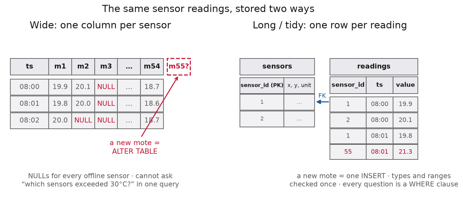
Fig. 5 The same sensor readings, stored two ways. In the wide layout, adding a sensor is a schema
change that ripples through every query that named the old columns; in the long layout it is a
single INSERT, and the sensor becomes a value you can filter on rather than a column name
you cannot.#
Read the long form back through the failures that sank the wide one and each is simply gone.
A new mote is one INSERT into sensors, after which its readings flow into the same
readings table as every other mote’s, no schema change in sight. A mote that goes offline
stops producing rows, which is honestly and visibly different from producing a row that
contains a zero. And “which sensors exceeded thirty degrees” is now WHERE value > 30, a
filter over rows the database already knows how to evaluate, because the sensor is a value in
a column and not the name of one. The wide table answered “what did all sensors read at this
instant” cheaply and answered everything else badly; the long table answers the questions you
actually keep asking of time-series.
A reasonable schema for this dataset is three tables:
CREATE TABLE sensors (
    sensor_id  int PRIMARY KEY,
    x_m        double precision,   -- location on the lab floor, metres
    y_m        double precision    -- static metadata: set once, not per reading
);

CREATE TABLE variables (
    variable   text PRIMARY KEY,   -- 'temperature', 'humidity', 'light', 'voltage'
    unit       text NOT NULL,      -- 'degC', '%RH', 'lux', 'V'
    lo         double precision,   -- plausible range, for validation
    hi         double precision
);

CREATE TABLE readings (
    sensor_id  int         NOT NULL REFERENCES sensors (sensor_id),
    ts         timestamptz NOT NULL,
    variable   text        NOT NULL REFERENCES variables (variable),
    value      double precision,
    PRIMARY KEY (sensor_id, ts, variable)
);
Notice where each fact has come to rest, because the placement is the design. A sensor’s
location is static, so it lives once in sensors. A quantity’s unit and its plausible range
belong to the quantity itself, not to any sensor or any moment, so they live in variables.
Only the measurements, which vary by sensor and by time, fill the large readings
table, and that table points back at the two small ones through foreign keys. This is the
fully tidy form, one row per (sensor, time, quantity), and its particular virtue is that
adding a new kind of measurement next semester is another row in variables rather than a
change to the shape of any table.
There is a common and entirely defensible middle ground you will meet, and it is not wrong:
collapse the variables idea back into typed columns, so that
readings has one row per (sensor, time) with a temperature double precision, a
humidity double precision, and so on. That form buys you a distinct, correct type for each
channel, and it halves nothing but the row count is a quarter of the tidy form’s. What it
costs is exactly what the tidy form buys: adding a channel is now an ALTER TABLE. Neither is
the “right” answer in the abstract; the assignment asks you to choose one and to say why, and
a good answer names the trade you made rather than pretending there wasn’t one.
Common pitfall
The reflex to build a wide “one column per sensor” table is the single most common mistake engineers make with sensor data, and you should resist it on purpose because it feels so natural. The tell is a table whose column names are entities: sensor ids, machine numbers, experiment run labels, well names. Whenever you catch yourself about to name a column after a particular thing you measured from, stop and put those things in rows instead. A column should be a kind of thing you measure. It should never be a particular thing you measured it from.
Types that carry physical meaning#
Because the schema is a contract, the column types are the clauses that carry the most weight, and two of them reward real thought on engineering data. The first is time, and it hides a surprise.
PostgreSQL offers two temporal types that look almost identical and behave very differently.
timestamp is a wall-clock reading with no zone attached, the database equivalent of a photo
of a clock on the wall: it tells you the hands said 2:30 but not which 2:30, in which place.
timestamptz is an instant in the actual history of the universe. The surprise, and it trips
up nearly everyone at first, is that despite its name timestamptz does not store a time
zone at all. It takes whatever zone-aware value you hand it, converts the instant to UTC,
stores the UTC instant, and forgets the zone entirely; on the way out it converts that instant
into whatever zone you ask to see it in. The name promises a stored zone and the
implementation delivers something better, a canonical instant that every client can render
locally. The practical rule that falls out of this is short: use timestamptz, and think of
your stored data as UTC. A bare timestamp of 2004-03-14 02:30:00 collected on a
clock-change night is ambiguous, naming a moment that either happened twice or never
happened, and no query can disambiguate it after the fact. The instant does not have that
problem, so ordering, differencing, and bucketing are all well defined regardless of where the
data was collected or where it is later analyzed.
Definition: timestamptz
timestamptz is PostgreSQL’s zone-aware timestamp, and despite its name it stores no zone: it converts the value to UTC, keeps that instant, and renders it back in whatever zone you ask to see it in. Use it, and think of your stored data as UTC.
Case study: the leap second of 30 June 2012#
It is easy to treat time as a solved problem and move on, and the clearest argument
against that is what happened at midnight UTC on the first of July, 2012. The
Earth does not rotate at a perfectly constant rate, so the world’s timekeepers occasionally
insert a leap second to keep atomic clocks aligned with the planet, and on this occasion the
final minute of 30 June was allowed to run to an unusual 23:59:60. A bug in the way the
Linux kernel handled that one extra second sent affected servers into a tight loop, pinning
their processors at 100 percent and hanging the services running on them. Reddit, LinkedIn,
Mozilla, Yelp, Foursquare, and StumbleUpon all reported outages that same night. The Amadeus
Altea reservation system, which sits under a large fraction of the world’s airline check-in,
was taken offline for about an hour, and staff at Qantas and Virgin Australia checked
passengers in by hand while it was down. An extra second, inserted on schedule and announced
years in advance, grounded people at airports.
The instructive detail is who did not fall over. Google had anticipated the problem and, in the hours around the leap second, deliberately smeared it across many tiny adjustments to its internal clocks, so that no server ever had to absorb a single discontinuous extra second, a technique it named the “leap smear.” The lesson for anyone who stores measurements generalizes cleanly and downward in scale. Calendar and clock arithmetic is a swamp of special cases, leap seconds and leap years and time zones and the twice-a-year hour that daylight saving adds or removes, and you do not want to be standing in it holding your own implementation. Store instants in UTC, give them a type the database understands, and let code that has already survived contact with every edge case do the arithmetic. The moment you decide to keep time as naive local strings and subtract them by hand, you have quietly volunteered to rediscover every one of those special cases yourself, in production, at 23:59:60.
numeric versus double precision#
The second choice is how to store the numbers, and the database does
not make floating point any less strange than it is anywhere else. double precision is a
64-bit binary float: fast, compact, and inexact. The classic demonstration, 0.1 + 0.2 coming
out as 0.30000000000000004, is as true inside PostgreSQL as it is in Python, because it is a
property of binary floating point and not of any particular language. numeric is an exact
decimal of arbitrary precision, which stores precisely the digits you wrote at the price of
being slower and larger. For physical sensor values the right default is double precision
without hesitation, because the uncertainty in the measurement itself dwarfs the floating-point
error by many orders of magnitude, and you will be averaging millions of these numbers where
compactness and speed matter. You reach for numeric when a value must be exact by definition
rather than by measurement: money is the textbook case, and a legally reportable calibrated
quantity is the engineering one. The interval type deserves a mention alongside them,
because it is a real duration rather than a number of seconds, which means ts - lag(ts)
hands you back an interval you can compare directly against '1 hour', with no unit
juggling and no chance of comparing seconds against milliseconds by accident.
A typed column is still not a validated column#
There is a trap for anyone who has just learned to trust types. A type constrains
the kind of value a column will hold, but it says nothing about whether a value of that kind
is possible. A double precision temperature column will accept 386 as cheerfully as 19,
because 386 is a perfectly good floating-point number; it is only an impossible temperature,
and impossibility is not a datatype. Catching it requires either a CHECK constraint declared
in the schema or a range filter written into your queries, and either way it requires you to
know something about the instrument that the type system cannot know for you. This dataset
makes the point with unusual clarity, and it hands you the very tool you need to do the
catching, sitting in plain sight in a column you might have dismissed as housekeeping.
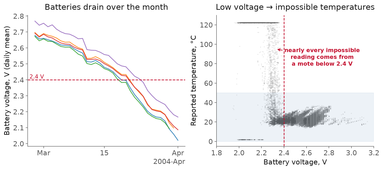
Fig. 6 The voltage channel is a data-quality signal, not just telemetry. As each mote’s
battery drains past roughly 2.4 V over the month (left), its temperature channel stops being
trustworthy and begins reporting physically impossible values (right). In this dataset about
27 percent of readings come from motes already below 2.4 V, roughly 18 percent of temperature
readings fall outside a generous 0-to-50-degree band, and essentially every one of those
impossible readings comes from a low-voltage mote.#
That the corruption lines up so precisely with low battery voltage is a small surprise: you
might have expected bad readings to be
scattered noise, and instead they are almost perfectly predicted by a second channel you were
recording anyway. The cleaning rule is therefore a fact the data hands you rather than a
judgment you have to defend: a reading taken while its mote was below 2.4 V is suspect, and voltage,
the channel you nearly ignored, is the context that tells you which numbers to trust. This is
exactly why the schema should carry its metadata explicitly, units and plausible ranges in
variables, per-mote calibration and location in sensors, and why storing that context
beside the values is an engineering requirement and not bookkeeping. A number without its
provenance can be believed but not checked.
SQL that answers engineering questions#
SQL is a language for describing the answer you want and leaving the database to work out how
to compute it, and that declarative character is easy to take
for granted. When you write a query you name the columns to return with SELECT, the table to
read them from with FROM, the rows to keep with WHERE, how to fold rows together with
GROUP BY, and which of the resulting groups survive with HAVING; joining reaches into
another table by matching keys. Nowhere in that do you say how to scan the disk, which order
to read rows in, or whether to use an index. You describe the result, and the query planner,
which we will meet properly in the indexing section, decides the mechanism. One consequence,
pleasant and slightly uncanny the first time you notice it, is that the very same query can run
by a completely different physical plan tomorrow, after the data has grown or an index has
appeared, with not a character of the query changed.
A word about the join, because every one in this session is written as a bare
JOIN and that is not the only kind. A plain JOIN is an inner join: it keeps
only the rows that match on both sides, and a row with no partner is not returned
at all. It does not come back with blanks, it is simply absent, and nothing warns
you. A LEFT JOIN instead keeps every row of the left-hand table and fills
NULL where the right-hand side had no match, which is what you want whenever the
left table is a list you need to be complete: a roster of sensors, a calendar of
days, a catalogue of parts. The difference is invisible until the day it matters,
and then it is the difference between “these five sensors dropped the most
readings” and “these five of the sensors that reported at all dropped the most” –
a sensor that never reported cannot be missing from a result it was never in.
Keep LEFT JOIN in mind for the assignment, and note that after one,
count(*) and count(some_right_column) are deliberately different numbers, for
the NULL reasons in the three-valued-logic section below.
Time bucketing is the workhorse of time-series SQL, and date_trunc is how you do it. It
rounds a timestamp down to a chosen granularity, the hour or the day or the minute, so that
grouping by the truncated value collapses a mess of irregular readings into tidy, regular
buckets. Hourly average temperature per sensor, the canonical first question anyone asks of
sensor data, is a single statement:
SELECT sensor_id,
       date_trunc('hour', ts) AS hour,
       avg(value)             AS avg_temp
FROM   readings
WHERE  variable = 'temperature'
GROUP  BY sensor_id, hour
ORDER  BY sensor_id, hour;
HAVING filters the groups rather than the rows, and the distinction is the thing beginners
most often trip on: WHERE runs before the grouping and sees
individual rows, HAVING runs after and sees aggregates. A dropout report is a natural use,
because a mote that fell silent is simply a mote whose reading count is suspiciously low:
SELECT sensor_id, count(*) AS n_readings
FROM   readings
WHERE  variable = 'temperature'
GROUP  BY sensor_id
HAVING count(*) < 30000      -- a healthy mote reports far more over a month
ORDER  BY n_readings;
The most powerful additions for time-series are window functions, because nothing else expresses “compare each reading to its neighbors” so directly. A window function computes across a set of rows related to the
current one without collapsing them into a group, so every reading keeps its own identity and
also gets to see the rows around it. lag reaches back to the previous reading, which turns
the reporting gaps that afflict every sensor network into an ordinary column you can filter
on:
SELECT sensor_id, ts,
       ts - lag(ts) OVER (PARTITION BY sensor_id ORDER BY ts) AS gap
FROM   readings
WHERE  variable = 'temperature';
Each mote aims to report about every 31 seconds, so any gap much larger than that is a
dropout, and now it is a dropout with a precise timestamp attached rather than an absence you
have to go looking for.
Definition: window function
A window function computes over a set of rows related to the current one without collapsing them into a group, so every row keeps its own identity while also getting to see its neighbors. lag, reaching back to the previous reading, is the workhorse for time-series.
A rolling average is the same machinery with an aggregate and a frame. Because the sampling is irregular, a frame defined by time is the honest choice rather than one defined by a fixed number of rows, and PostgreSQL lets you write almost exactly that:
SELECT sensor_id, ts, value AS voltage,
       avg(value) OVER (
           PARTITION BY sensor_id ORDER BY ts
           RANGE BETWEEN INTERVAL '1 hour' PRECEDING AND CURRENT ROW
       ) AS voltage_1h_avg
FROM   readings
WHERE  variable = 'voltage';
Filtering for the impossible values from the previous section is a plain WHERE, and joining
to sensors attaches the location that makes a result interpretable rather than a bare list of
numbers:
SELECT r.sensor_id, s.x_m, s.y_m, r.ts, r.value
FROM   readings r
JOIN   sensors  s USING (sensor_id)
WHERE  r.variable = 'temperature'
  AND (r.value < 0 OR r.value > 50);   -- outside the plausible indoor band
CASE lets you label a value rather than discard it, which is very often what you actually
want, since a suspect reading you have flagged is more useful than one you have silently
dropped: CASE WHEN value BETWEEN 0 AND 50 THEN 'ok' ELSE 'suspect' END turns the same test
into a column you can then group on and count. Treat all of this as a vocabulary to recognize
rather than a list to memorize; the demo strings these pieces together against the live
database, and fluency comes from writing them, not from reading them.
Getting data in: COPY, psql, and Python#
A schema is an empty promise until you load it, and how you load matters far more than it
first appears. The obvious way, especially from Python, is a loop that issues one INSERT
per row, and on a dataset like this one that is a quiet catastrophe: two million separate
statements, each a round trip to the server with its own transaction overhead, turning a job
that should take seconds into one that takes an afternoon. The right way is COPY,
PostgreSQL’s bulk loader, which streams an entire file into a table in a single operation and
routinely runs two or three orders of magnitude faster.
Definition: COPY
COPY is PostgreSQL’s bulk loader: it streams an entire file into a table in one operation, routinely two or three orders of magnitude faster than a loop of one INSERT per row.
COPY readings (sensor_id, ts, variable, value)
FROM '/data/readings.csv' WITH (FORMAT csv, HEADER true);
psql, the command-line client, is where you run this interactively and then poke at what
landed; its \copy variant performs the same load from the client side when the file lives on
your machine rather than the server’s. From Python the two paths are
psycopg, the direct PostgreSQL driver, whose copy
interface exposes that same fast path, and SQLAlchemy, which
adds a layer that lets the same code target different databases and interoperates with pandas
through to_sql and read_sql. The demo uses both, psycopg for the bulk load and
SQLAlchemy for reading query results back into dataframes.
Real data resists the loader, and this dataset resists it in exactly the ways real sensor
exports do, which is the reason it was chosen. Its raw file has rows truncated to a handful of
fields where a transmission was cut off, timestamps carrying sub-second precision, and, in a
detail that surprises students every time, moteid values outside the documented range of 1
to 54. There are supposed to be 54 motes; the file contains a scattering of readings tagged
with ids well above that, corruption not in the measurements but in the identifier itself. The
professional response is a staging table: COPY the raw text into a permissive table with
forgiving types, then clean and validate with SQL as you insert into the real readings
table, so that the cleaning rules are written down as queries anyone can read rather than
buried in a one-off script. “Discard readings from motes below 2.4 volts” and “reject any row
whose sensor_id is not in the roster” become WHERE clauses on that transfer, and for the
corrupt mote ids you do not even have to write the rule, because the foreign key to sensors
rejects them for you the moment you try to insert one.
Making range queries fast: indexes and EXPLAIN ANALYZE#
The query that dominates time-series work, once the schema is right and the data is in, is the range scan: one sensor, one window of time. Without help, the database answers it the only way it can, by reading every row in the table and throwing away the ones that do not match, a sequential scan whose cost grows with the size of the whole table even when the answer is a hundred rows out of nine million. An index is a secondary structure that lets the database find the matching rows without reading everything else. PostgreSQL’s default is a B-tree, which keeps keys in sorted order, so a range lookup becomes a descent to the start of the range followed by a walk along it, and its cost tracks the size of the result rather than the size of the table.
Definition: database index
A database index is a secondary structure that lets the database find matching rows without reading the whole table. PostgreSQL’s default is a B-tree, which keeps keys in sorted order, so a range lookup costs the size of the result rather than the size of the table.
For per-sensor time-range queries the index you want is a composite B-tree on (sensor_id, ts), in that order, because it groups each sensor’s readings together and keeps them sorted by
time, which is precisely the access pattern. The effect is not marginal.
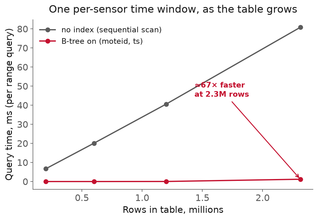
Fig. 7 The same query, counting one sensor’s readings in a one-hour window, as the table grows toward 2.3 million rows. The sequential scan’s cost climbs in step with the table; the B-tree index barely moves, roughly 65 times faster at full size. Measured in SQLite, which uses B-trees as PostgreSQL does, so the figure needs no running server; the demo reproduces the same result live in PostgreSQL.#
The tool for watching this happen is EXPLAIN ANALYZE, which runs your query and prints the
plan the database actually chose, annotated with real timings. It is intimidating at first
because it is a tree and the tree is dense, but you can read almost everything you need from
two places: the scan at the base of the plan, which names the strategy (Seq Scan versus
Index Scan or Index Only Scan), and the total execution time at the bottom. Run it on the
same query before and after building the index:
EXPLAIN ANALYZE
SELECT count(*) FROM readings
WHERE  sensor_id = 1
  AND  ts BETWEEN '2004-03-15' AND '2004-03-16';
Before the index the readings are read by a sequential scan and the time scales with the
table; on the full dataset in the demo this lands around 190 milliseconds. After
CREATE INDEX ON readings (sensor_id, ts) the same query becomes an Index Only Scan and the
time collapses to a few hundredths of a millisecond. There is a lesson hiding inside that
composite index: if you
had made (sensor_id, ts, variable) the primary key, as the schema above recommends, this
index would already exist, because a primary key is an index, and this one begins with
exactly the columns the query filters on. Choosing your key well hands you your most important
index for nothing. The demo deliberately starts from a table without that key so the change is
visible, but in a real schema the integrity constraint and the performance structure are often
the same object seen from two sides.
Definition: EXPLAIN ANALYZE
EXPLAIN ANALYZE runs your query and prints the plan the database actually chose, annotated with real timings. Read two places: the scan at the base of the plan (Seq Scan versus Index Scan) and the total execution time at the bottom.
Indexes are emphatically not free, and it matters to say so, because the beginner’s instinct
after seeing that speedup is to index everything. Each index costs storage, and, more
importantly, each one slows down every write, because the index has to be updated on every
insert and update, so a table with six indexes does roughly six times the bookkeeping on each
new row. An index the planner never chooses is pure overhead with no benefit at all. The
discipline is to index the access patterns you actually have, then confirm with
EXPLAIN ANALYZE that the planner is in fact using them, because the planner is a
cost-estimating optimizer and it will rationally ignore an index it judges unhelpful, for
instance on a column with only a handful of distinct values where a scan is cheaper.
When per-time access dominates at real scale, a purpose-built extension pays off. TimescaleDB turns an ordinary PostgreSQL table into a hypertable that is transparently partitioned into time-based chunks, so that a query for last week touches only last week’s chunks and old data can be compressed or dropped a whole chunk at a time. It is the same SQL over the same relational model, tuned for the particular shape of time-series. Know it exists before the day you need it.
Where the relational model pushes back#
Everything to this point has been an argument for the relational database, and it is a strong argument, but a course that only ever praised its default tool would be teaching advocacy rather than engineering. The relational model is a default, not a universal answer, and the mature version of this knowledge is knowing where it strains and what you reach for when it does. Learn several of its limits before you meet them under deadline.
The schema is rigid, and rigidity has a price#
The same schema that protected your data is expensive to change once the table is
large. Adding or altering a column with ALTER TABLE can, depending on the change and the
database, lock the table or rewrite it row by row; historically, adding a column with a
non-constant default rewrote the entire table, and while PostgreSQL has optimized the common
cases, the general problem remains. Running a migration against a nine-million-row readings
table in the middle of a live deployment is a real operation with real risk, and serious shops
manage it with migration tooling and versioning rather than ad-hoc ALTER statements. Where
the data itself is heterogeneous, experiment metadata in which every run records a different
and unpredictable set of fields, the rigid schema stops helping and starts fighting you, and
this is exactly the territory where document stores earn their place.
NULL is not a value, and three-valued logic will surprise you#
SQL does not have two truth values but three: true, false, and unknown. NULL means “unknown,”
and any comparison involving it yields not true or false but NULL itself, and this produces
results that look like bugs until you internalize the rule. value = NULL is never true, which
is why you must write value IS NULL; a filter like WHERE value <> 30 silently drops every
row where value is null, because “unknown is not equal to 30” evaluates to unknown, not to
true; and NOT IN against a subquery that contains a single null returns no rows at all, a
notorious footgun. The aggregate functions have their own version of this:
count(*) counts rows while count(value) counts only the non-null ones, and avg(value)
averages only the readings that are present, so a mote that dropped half its readings is not
penalized in an average unless you have separately counted how many it reported. None of this
is a defect in PostgreSQL. It is the defined semantics of SQL, and it quietly produces wrong
analyses for anyone who forgets it.
Definition: three-valued logic
SQL has three truth values, not two: true, false, and unknown. NULL means unknown, and any comparison with it yields unknown, which is why value = NULL is never true and you must write value IS NULL.
Floating point in a column is still floating point#
Putting a number in a double precision column does not make it exact, and the problem here
has a sharp edge for reproducibility. Because floating-point addition is not associative, the
result of avg or sum over a large column can depend on the order in which the rows were
summed, and when PostgreSQL parallelizes an aggregate across worker processes, as it did in the
EXPLAIN example above, that order is not deterministic between runs. The differences live in
the last digits and sit far below any sensor’s measurement noise, so for this course’s work
they are harmless, but they are real, and they ambush people who expected the database, of all
things, to give back exactly the same number every time.
Normalization trades write-simplicity for read-cost#
The clean, normalized schema that made corrections safe also means that answering a question
about a sensor’s location requires a join back to the sensors table, and in a heavily
normalized design a single natural question can require joining across many tables at once.
Joins across large tables are exactly where query time tends to go, and the standard remedy,
denormalization, which duplicates some columns to avoid the join, reintroduces precisely the
update anomalies that normalization existed to prevent. So even the design principle at the
heart of the relational model is a trade rather than a free lunch: you are choosing where to
pay, in write-time consistency or in read-time joins, not whether to pay at all.
Even our recommended shape has costs#
Honesty obliges turning this lens on our own recommendation. The fully tidy (sensor_id, ts, variable, value) form quadruples the row count, from 2.3 million readings to more than nine
million rows in the demo, which is not free in storage or in scan time. It forces every
measurement into a single double precision column, so a temperature and a categorical status
flag cannot have different types even though they obviously should. It makes a per-variable
CHECK constraint awkward to express, because one column now holds several physically
different quantities. And it puts a WHERE variable = '...' on very nearly every query you
will ever write. The typed-column alternative escapes all of these and pays for the escape
with schema rigidity. Every shape costs something. Choose the costs you pay on purpose.
Row stores are the wrong tool for wide analytical scans#
The deepest limitation is structural. A relational database like PostgreSQL is a row store: it keeps all of a row’s columns together on disk. That layout is ideal for the transactional pattern of reading or writing whole rows, and it is close to the worst possible layout for the analytical pattern of scanning a single column across the entire history, because to read one column out of many the database must still pull every column of every row off the disk to get at it. Our index win was for a selective query that touched a hundred rows; a full analytical aggregate over one channel of the whole table reads everything, and no index rescues a query that needs all the rows. This single fact is why a relational online transaction processing (OLTP) database is not the end of the storage story, and it is exactly the problem that columnar formats and embedded analytical engines are built to solve.
Definition: row store
A row store like PostgreSQL keeps all of a row’s columns together on disk. That is ideal for reading and writing whole rows, and close to the worst layout for scanning one column across the whole history, because it must pull every column of every row off the disk to reach the one it needs.
Writes scale up but not easily out, and the server has weight#
A single PostgreSQL primary serves one stream of writes. You can scale reads by adding
replicas, but scaling writes beyond one machine means sharding, partitioning the data
across servers, and sharding a relational database while preserving cross-shard joins and
transactions is one of the hard problems in the field, hard enough that the entire
NoSQL movement grew up around avoiding it. High-ingest sensor and internet of things (IoT) systems, taking millions
of writes a second, are where specialized time-series and distributed stores live; partitioning
and TimescaleDB raise the ceiling considerably but do not remove it. And underneath all of this
is plain operational weight: a relational database is a server you must run, secure, back up,
monitor, and connect to within its connection limits, which is real overhead that a CSV file or
an embedded engine like SQLite or DuckDB simply does not carry. And “SQL” is a family of
dialects rather than a single language, so date_trunc, the exact
window-frame syntax, and the type names all differ between PostgreSQL, MySQL, SQLite, and the
rest, and moving a non-trivial query from one to another is work, not a copy and paste.
What a practitioner should take from this
Choose the relational database when correctness under concurrent writes, referential integrity, and flexible ad-hoc querying are what dominate, which for continuously arriving, interrelated engineering data is most of the time. Reach past it deliberately when your access pattern is wide analytical scans, where a column store wins; when your data is schema-heterogeneous, where a document store fits; or when your write volume outgrows a single machine, where distributed and time-series systems come in. The skill is matching the store to the access pattern rather than staying loyal to one tool.
In-class demo#
We bring up PostgreSQL in Docker from a provided docker-compose.yml, create the
sensors, variables, and readings schema from this session, and COPY the month of Intel
Lab readings in. Then we answer the engineering questions live: hourly average temperature per
sensor with date_trunc, the motes with the most dropped intervals via a windowed lag, a
rolling voltage average over a time-based frame, and the impossible temperatures that low
battery voltage predicts, which the notebook confirms with a join. The moment to watch for is
the index. We run the same per-sensor range query under EXPLAIN ANALYZE before and after
creating the B-tree on (sensor_id, ts), and read the plan change from a sequential scan to an
Index Only Scan together, along with the execution time falling from around 190 milliseconds
to a few hundredths of one.
The runnable notebook is l03-sql-timeseries.ipynb. It expects the
database from the compose file; start it before class if you would like to follow along on your
own machine.
Summary#
A relational database belongs in an engineering data platform because it is a contract you
can query. Modeling sensor readings in the long form, keyed by sensor and time with the static
metadata normalized into sensors and variables, makes a new sensor an INSERT rather than
a migration and turns every comparative question into a WHERE clause. Choosing types with
physical meaning, timestamptz understood as UTC and double precision for measured values,
closes off a category of time and precision bugs, though the leap-second night is a reminder
that time punishes the overconfident and the 386-degree readings are a reminder that a type is
not a validation. SQL’s GROUP BY, date_trunc, and window functions answer the questions you
actually have about time-series, COPY gets the data in quickly, and a B-tree on (sensor_id, ts), confirmed with EXPLAIN ANALYZE, turns the dominant range query from a full scan into a
seek. And because no tool is universal, the honest close is the list of places the relational
model pushes back, from three-valued NULL logic to the row store’s poor fit for wide
analytical scans, each one a reminder that the relational database is a strong default rather
than a universal answer.
Resources#
PostgreSQL Tutorial. The official walk-through from
CREATE TABLEto joins and aggregates; the fastest way to get fluent if SQL is new to you.PostgreSQL: Joins Between Tables. Inner against outer joins in two pages of worked examples. Read it before the assignment: a
LEFT JOINis the only way to see a sensor that never reported.PostgreSQL: Window Functions. The tutorial chapter on
OVER,PARTITION BY, and frames, which are the part of SQL that makes time-series tractable.PostgreSQL: Date/Time Types. Read the
timestampversustimestamptzdistinction here, and the note that the latter stores UTC rather than a zone, before you design a schema.PostgreSQL: Numeric Types. The exact-versus-float trade-off, from the authority on it.
PostgreSQL: Date/Time Functions.
date_truncand its neighbors, the time-bucketing toolkit.PostgreSQL: COPY. The bulk loader, and the reason your import should not be a loop of
INSERTs.PostgreSQL: Using EXPLAIN. How to read a query plan; start with the scan at the base and the total time.
PostgreSQL: Indexes. What a B-tree index is, when a multicolumn index helps, and when an index is dead weight.
Intel Lab Data. The dataset used all week: schema, download, and the note that the readings are noisy and the batteries fail. Served over plain HTTP.
Leap second bug cripples Linux servers at airlines, Reddit, LinkedIn. The Register’s contemporaneous account of 30 June 2012, and the source of the outage list above.
TimescaleDB: Hypertables. The time-series extension to PostgreSQL; read the overview, not the whole manual.
Codd, “A Relational Model of Data for Large Shared Data Banks,” CACM 1970. The founding paper, and still the clearest statement of why logical structure should be independent of physical storage.
Kleppmann, Designing Data-Intensive Applications, Chapter 3 (“Storage and Retrieval”). The clearest single explanation of why row stores and column stores make opposite choices.
DuckDB: Reading and Writing Parquet Files. SQL over columnar files with no server at all.
Assignment#
Assignment 1, the reproducible project scaffold, is due 08-31-2026. This session’s schema design, SQL, and indexing are the foundation of Assignment 2, the module’s databases assignment, which asks you to model the Intel Lab data, load it into PostgreSQL, and answer a set of engineering queries with SQL. This is a pointer, not the rubric.
Practice module#
Practice module for this session, about ten minutes of questions drawn from the schema decisions, the queries and the indexing results above. It runs entirely in your browser, the questions are selected from your Andrew ID, and it ends by producing a PDF you upload for participation credit.