Lecture 15: Bayesian optimization

At a glance

• Session Lecture 15, Week 8

• Arc Machine learning and deep learning

• Slides Deck for this session

• Practice Practice module for this session

• Demo l15-bayesian-optimization.ipynb, Bayesian optimization of a reactor in BoTorch: one knob, then two, against random search

• Tools BoTorch, on PyTorch and GPyTorch

Why this matters

• Some functions cost a lot to evaluate. One evaluation is a lab experiment, a pilot-plant run, a day of simulation, a battery cycled to failure.

• You can afford tens of evaluations, not thousands.

• There is no formula and no gradient: you set the inputs, you wait, you get one number back, with noise.

• Gradient-based optimizers need many cheap evaluations. Grid search and random search waste the few you have.

• Bayesian optimization (BO) uses every past evaluation to decide the next one. On today’s reactor it finds the best operating point in about 8 experiments; random search does not get there in 30.

Learning objectives

By the end of this session you should be able to:

• Explain what Bayesian optimization (BO) is, why it is called Bayesian, and when it beats gradient-based and other derivative-free optimizers: expensive, noisy, black-box objectives with a budget of tens of evaluations.

• Explain the BO loop (a Gaussian-process surrogate, an acquisition function, evaluate, update) and the trade-off between exploration and exploitation.

• Write and compute the common acquisition functions: probability of improvement (PI), expected improvement (EI) and upper and lower confidence bounds (UCB, LCB), and explain how their parameters set the balance between exploration and exploitation.

• Run BO in BoTorch on an engineering problem and compare it with random search over several seeds.

• Name the extensions engineers need (constraints, batches, several objectives, several fidelities) and recognize where BO is used across engineering and science.

The problem: a few expensive experiments

The example: making B, not C

• A raw material A turns into the product we sell, B.

• B is not the end of the road: left in the hot tank, it keeps reacting into a waste, C.

\[ \text{A} \;\xrightarrow{\;k_1\;}\; \text{B} \;\xrightarrow{\;k_2\;}\; \text{C} \]

• Heat speeds up both steps, but it speeds up the second one more.

  • Too cold: A barely reacts. Little B.

  • Too hot: B forms fast and burns into C even faster. Little B.

  • In between: a best temperature.

• Think of toast, or of roasting coffee: heat turns raw into good, then good into burnt.

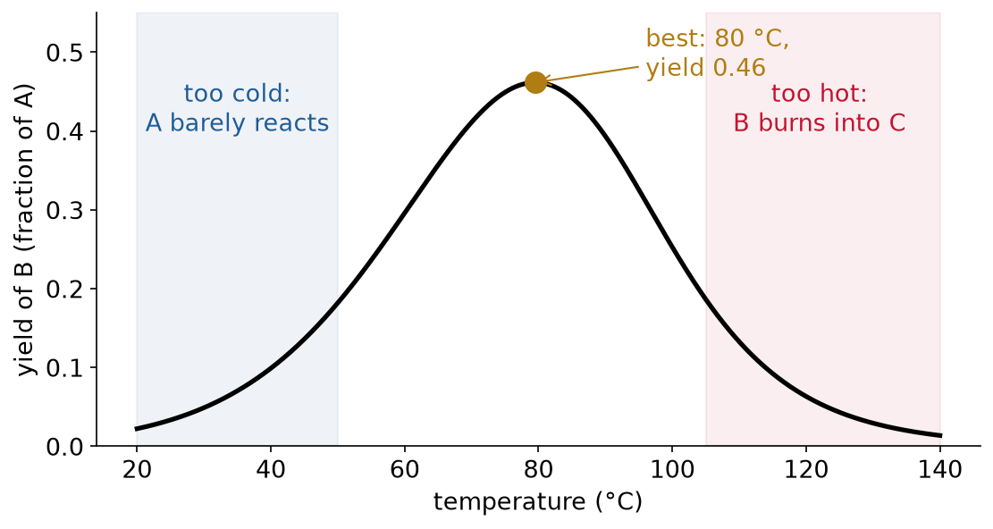
Fig. 111 The yield of B against temperature, with 10 minutes in the tank. The best is 0.46 at 80 °C. In the lab nobody sees this curve: each point on it is one experiment.

• The yield is the fraction of A that leaves the tank as B. At steady state in a stirred tank:

\[ y = \frac{k_1 \tau}{(1 + k_1 \tau)(1 + k_2 \tau)} \]

• \(\tau\): the residence time, how long the liquid stays in the tank (min).

• \(k_1\), \(k_2\): rate constants (1/min), from Arrhenius’ law, \(k_i = k_{i,\text{ref}}\, e^{-E_i/R\,(1/T - 1/T_\text{ref})}\).

• The second step has the larger activation energy: \(E_2 = 110\) kJ/mol against \(E_1 = 60\) kJ/mol. That is what makes heat hurt eventually.

• We use the formula only to play the role of the lab and to check answers. The optimizer never sees it.

The same shape in industry

The product is made in the middle of a chain and destroyed by going further:

• Ethylene oxide, the raw material for antifreeze and many plastics: ethylene is partly oxidized on a silver catalyst, and over-oxidation burns it to CO₂ and water. The selectivity to ethylene oxide is the number the operators watch (Pu et al., 2019).

• Sugar from wood: acid breaks cellulose into glucose, and the glucose breaks down further into waste. Saeman (1945) modeled it as two consecutive first-order reactions, exactly A → B → C, so the sugar yield has a maximum.

• Drug synthesis: the drug is often an intermediate, and over-reaction makes impurities. Choosing the conditions that maximize the yield is exactly what BO was used for by Shields et al. (2021), below.

Why the budget matters

• Each experiment takes hours: heat the tank, wait for steady state, take a sample, analyze it.

• With one knob (temperature), a grid of 1 °C steps from 20 to 140 °C is 121 experiments.

• With two knobs (temperature and residence time) on a modest grid, thousands.

• Random search spends experiments where nothing interesting happens.

Definition: black-box objective

A black-box objective is a function you can only evaluate: set the inputs, run the experiment or simulation, read one (noisy) number. No formula, no gradient.

Gen 0 and Gen 1: machine learning with intention

In Lecture 13 we met generations of machine learning in engineering:

• Gen 0: a surrogate model replaces an expensive simulator. It predicts. That is all.

• Gen 1: the surrogate “knows what it does not know”: it also says how uncertain it is, and that uncertainty decides where to run the next experiment or simulation. Machine learning with intention.

Bayesian optimization is Gen 1. The idea goes back to Kushner (1964) and Močkus (1975), and became standard with Jones, Schonlau and Welch (1998).

Why it is called Bayesian

• Bayesian statistics treats what we do not know as a probability distribution, and updates it with data.

• Here, what we do not know is the function itself: the yield at every temperature.

\[ \underbrace{p(f \mid \text{data})}_{\text{posterior}} \;\propto\; \underbrace{p(\text{data} \mid f)}_{\text{likelihood}} \;\cdot\; \underbrace{p(f)}_{\text{prior}} \]

• Prior \(p(f)\): what we believe before any experiment. “The yield is somewhere around 0.25, and it changes smoothly over about 20 °C.”

• Likelihood \(p(\text{data} \mid f)\): how well a candidate curve \(f\) explains the measurements, given the noise (0.01). We measured 0.181 at 50 °C: a curve through 0.18 there fits, a curve through 0.40 does not.

• Posterior \(p(f \mid \text{data})\): what we believe after the experiments. Only curves that fit the data remain: after 30 and 50 °C, every curve passes near 0.05 and 0.18; at 110 °C, anything is still possible.

• A Gaussian process (GP) is a prior over functions for which this update is exact and cheap. Lecture 14 built it: a mean \(\mu(x)\) and an uncertainty \(\sigma(x)\) at every input.

• Every experiment pinches the band where it was run. Far from the data, the band stays wide.

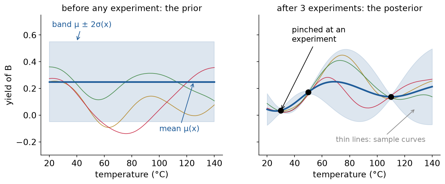
Fig. 112 A GP before and after three experiments, with fixed settings (mean 0.25, standard deviation 0.15, length scale 20 °C). Thin lines: sample curves from each.

• Then the decision is taken on the posterior: where to experiment next, given what we now believe.

• Bayesian optimization = a Bayesian belief about the function + a decision on that belief. “The term Bayesian optimization was coined in the seventies”, citing Močkus, Tiesis and Žilinskas (1978) (Shahriari et al., 2016, p. 17).

Definition: surrogate model

A surrogate model is a cheap model of the objective, fitted to the evaluations so far. In BO it is usually a GP, because it returns both a prediction \(\mu(x)\) and an uncertainty \(\sigma(x)\).

The Bayesian optimization loop

Definition: Bayesian optimization (BO)

Bayesian optimization maximizes a black-box objective in few evaluations: fit a surrogate to every evaluation so far, choose the next input by maximizing an acquisition function, evaluate it, and repeat.

Definition: acquisition function

An acquisition function \(a(x)\) scores every candidate input by how useful it would be to evaluate it next. It is computed from the surrogate, so it is cheap. The next experiment is its maximizer.

The loop:

1. Fit the GP to every experiment so far.

2. Score every candidate with the acquisition function.

3. Run the experiment where the score is largest.

4. Add the result to the data, and repeat until the budget is spent.

Terminology

• Incumbent \(f^*\): the best value measured so far.

• Budget: the number of evaluations you can afford.

• Regret: the gap between the best possible value and the best one found. BO tries to make it small with few evaluations.

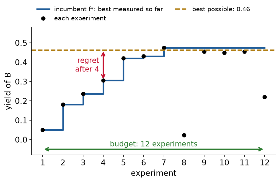
Fig. 113 The worked example’s twelve experiments. The incumbent (blue) is the best measured yield so far. After 4 experiments the regret is 0.46 − 0.31 = 0.16; after 7 it is about zero.

The loop on the reactor

• Start: two old runs from the lab notebook, both on the cold side, at 30 and 50 °C.

• BO with expected improvement then picked, one at a time: 54, 61, 72, 87, 81 °C.

• Experiment 8 jumped to 140 °C: the GP was still unsure there, so the expected improvement there was not zero. The yield was 0.02, and the band collapsed there.

• Then it settled at 80 °C. It reached 98% of the best possible yield at experiment 7.

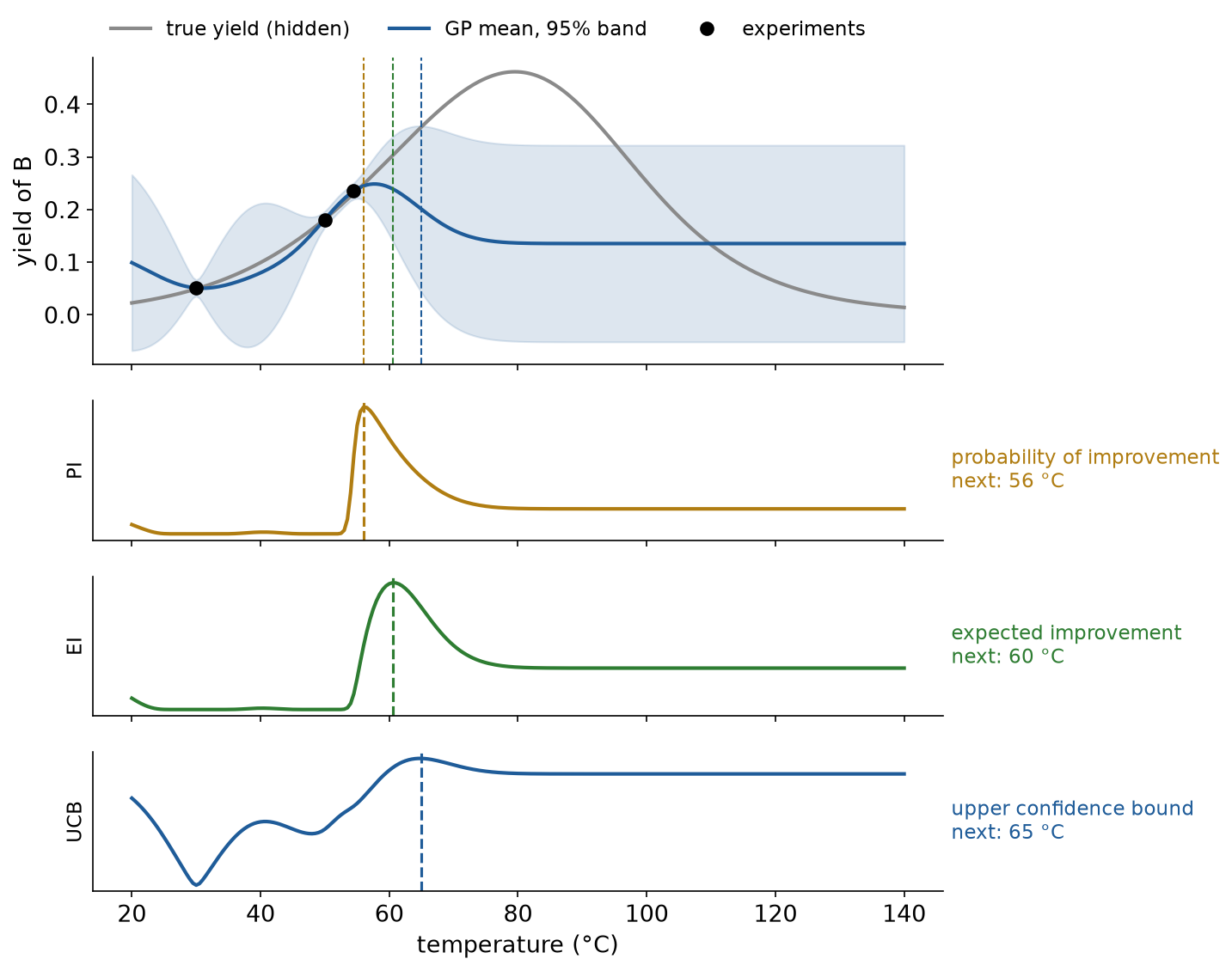
Fig. 114 One GP after three experiments, and three acquisition functions. Each picks a different next temperature: 56, 61 and 65 °C.

Exploration and exploitation

Definition: exploitation and exploration

Exploitation runs the next experiment where the surrogate predicts a good value (high \(\mu\)). Exploration runs it where the surrogate is unsure (high \(\sigma\)).

• Pure exploitation keeps sampling next to the best point so far. It can sit on a local optimum forever, because it never looks elsewhere.

• Pure exploration samples wherever the band is widest. That is close to a careful random search: it learns the whole curve and ignores the goal.

• Every acquisition function is a recipe for the balance between the two, with a knob: \(\kappa\) in UCB, \(\xi\) in PI and EI.

Acquisition functions

All of them use the GP’s mean \(\mu(x)\) and standard deviation \(\sigma(x)\), and the incumbent \(f^*\).

Definition: z-score

The z-score is how many GP standard deviations the predicted value \(\mu(x)\) sits above the best so far. \(z > 0\): the GP expects to beat \(f^*\). \(z < 0\): it expects to fall short.

\[ z = \frac{\mu(x) - f^* - \xi}{\sigma(x)} \]

• \(\xi \ge 0\) (xi): a margin, the smallest gain that counts. With \(\xi = 0.01\), a temperature counts as an improvement only if it beats the best yield by more than 0.01.

• A larger \(\xi\) ignores tiny gains right next to \(f^*\), so the search moves away from it: more exploration. The worked example uses \(\xi = 0\).

• Reactor, at 60 °C after 3 experiments: \(\mu = 0.242\), \(\sigma = 0.046\), \(f^* = 0.236\), so \(z = 0.13\).

Probability of improvement (PI)

Definition: probability of improvement

Probability of improvement (PI) is the probability that the value at \(x\) beats the best so far by more than \(\xi\).

\[ \text{PI}(x) = P\big(f(x) > f^* + \xi\big) = \Phi(z) \]

PI in four steps, on the reactor at 60 °C after three experiments:

1. The GP does not give one yield at 60 °C but a bell of possible yields: normal, with mean \(\mu = 0.242\) and standard deviation \(\sigma = 0.046\).

2. The best yield so far is \(f^* = 0.236\).

3. PI is the share of the bell above \(f^*\): 0.55, so a 55% chance that 60 °C beats the best so far.

4. The same number from \(z\): \(z = (0.242 - 0.236)/0.046 = 0.13\), and \(\Phi(0.13) = 0.55\). \(\Phi(z)\), the standard normal cumulative distribution, is the share of a standard bell to the left of \(z\), a number from 0 to 1.

• Pro: a probability, easy to read.

• In short: PI runs the experiment most likely to beat the best so far, however small the gain.

• Con: it ignores how much better. With \(\xi = 0\) it picks a point just above the incumbent, with a high chance of a tiny gain: it exploits. A point next to \(f^*\) with a narrow bell gets PI near 1 for a gain of almost nothing.

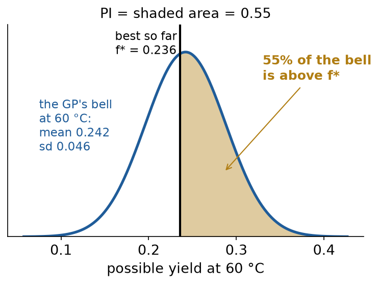
Fig. 115 The GP’s belief about the yield at 60 °C after three experiments: a bell with mean 0.242 and standard deviation 0.046. PI is the share of the bell above the best so far, 0.236: 0.55.

Expected improvement (EI)

Definition: expected improvement

Expected improvement (EI) is the average amount by which the value at \(x\) beats the best so far, counting a miss as zero.

The improvement at \(x\) is \(I(x) = \max(f(x) - f^*, 0)\): zero if we do not beat the incumbent. EI is its expected value under the GP:

\[ \text{EI}(x) = \mathbb{E}\big[I(x)\big] = \underbrace{(\mu - f^*)\,\Phi(z)}_{\text{exploitation: high } \mu} + \underbrace{\sigma\,\phi(z)}_{\text{exploration: high } \sigma} \]

• \(I(x)\), the gain: if the yield at \(x\) turns out to be \(f\), the gain is \(f - f^*\); below \(f^*\), the gain is 0.

• \(\mathbb{E}\), the average: average the gain over the GP’s bell of possible yields.

• \((\mu - f^*)\,\Phi(z)\), the exploitation term: how far the mean is above \(f^*\), times \(\Phi(z)\), the chance of beating \(f^*\) (as in PI). Large where \(\mu\) is high.

• \(\sigma\,\phi(z)\), the exploration term: the bell’s width \(\sigma\) times \(\phi(z)\), the height of the standard bell at \(z\) (the standard normal density). Large where \(\sigma\) is large.

• With \(\xi = 0\), \(z = (\mu - f^*)/\sigma\).

• The first term grows where the mean is high, the second where the uncertainty is high.

• EI is zero at an experiment already run (no uncertainty, no improvement) and grows away from the data.

• It is usually credited to Močkus and colleagues in the 1970s; Garnett (2023) traces it to Šaltenis (1971). Jones, Schonlau and Welch (1998) made it the default (see EGO, below).

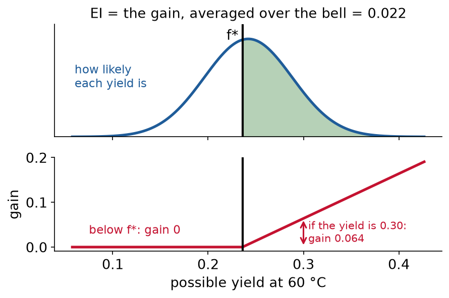
Fig. 116 EI at 60 °C after three experiments. Top: how likely each possible yield is. Bottom: the gain each possible yield would bring, zero below \(f^*\). EI is the gain averaged over the bell: 0.022.

Log expected improvement (LogEI)

Definition: LogEI

LogEI computes \(\log \text{EI}\) directly, with formulas that stay accurate where EI is tiny. It has the same maximizer as EI: the logarithm does not move the peak.

Why it was created: far from the data, EI is so small that the computer rounds it to exactly 0 (underflow). Ament et al. (2023) found that EI’s values “vanish numerically in many regions”, which makes EI hard to maximize (paper). What the figure below shows, on the reactor after its 12 experiments:

• Top: EI. One narrow peak near 80 °C, about \(10^{-8}\) high.

• Red: the temperatures where the computer stores EI as exactly 0 (12% of them). There EI is flat, so the optimizer of the acquisition, which follows its slope, has no direction to move.

• Bottom: \(\log \text{EI}\). A finite number everywhere, down to about \(-1100\), sloping up toward 80 °C.

• Both peak at the same temperature, so both pick the same next experiment. BoTorch’s LogExpectedImprovement is what the worked example uses.

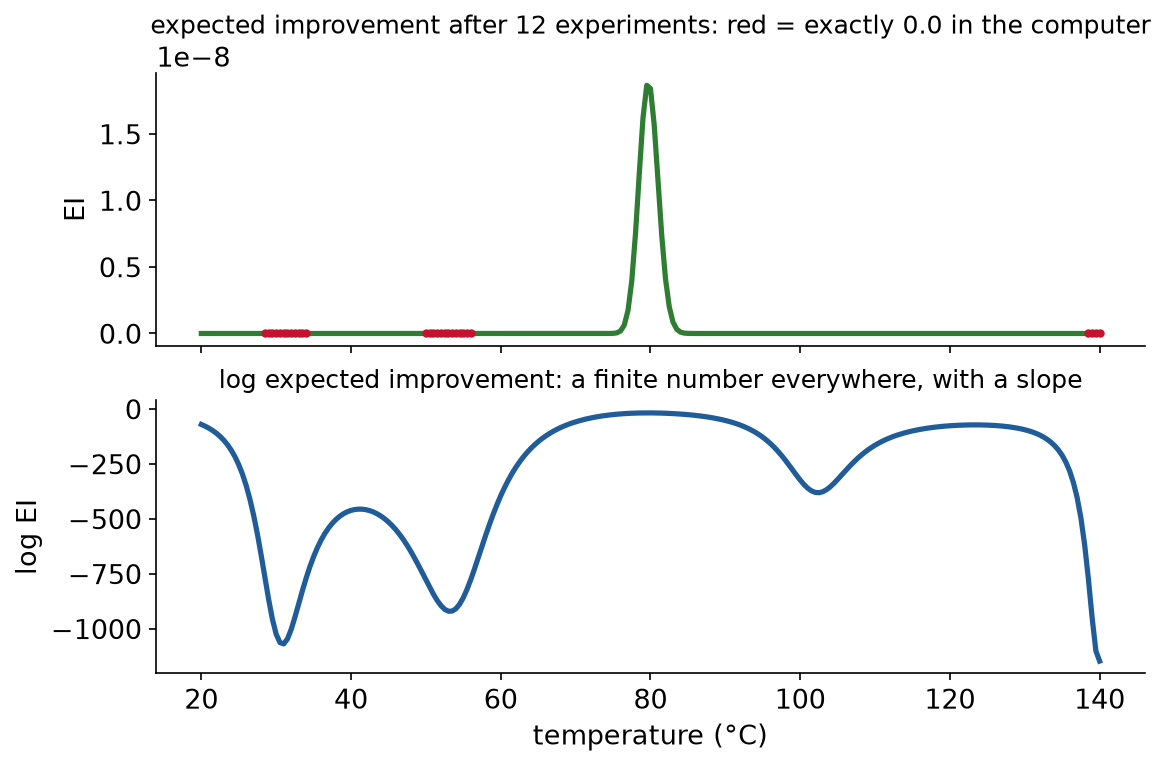
Fig. 117 The GP after the worked example’s twelve experiments. Plain EI (top) is exactly zero in the red regions; log EI (bottom) is finite everywhere.

Upper and lower confidence bounds (UCB, LCB)

Definition: upper confidence bound

The upper confidence bound (UCB) is an optimistic score: the GP mean plus \(\kappa\) standard deviations. The lower confidence bound (LCB), \(\mu - \kappa\sigma\), is the same idea for minimizing.

\[ \text{UCB}(x) = \underbrace{\mu(x)}_{\text{expected value}} + \underbrace{\kappa}_{\text{knob}}\,\underbrace{\sigma(x)}_{\text{uncertainty}} \qquad \text{LCB}(x) = \mu(x) - \kappa\,\sigma(x) \]

• \(\kappa\) (kappa): how many standard deviations of optimism. UCB scores each input by the top of its band, \(\mu + \kappa\sigma\).

• \(\kappa\) is the knob. \(\kappa = 0\): the mean only, pure exploitation. Large \(\kappa\): the band wins, exploration.

• \(\kappa = 2\) is the top of the 95% band. On the reactor it picks 65 °C.

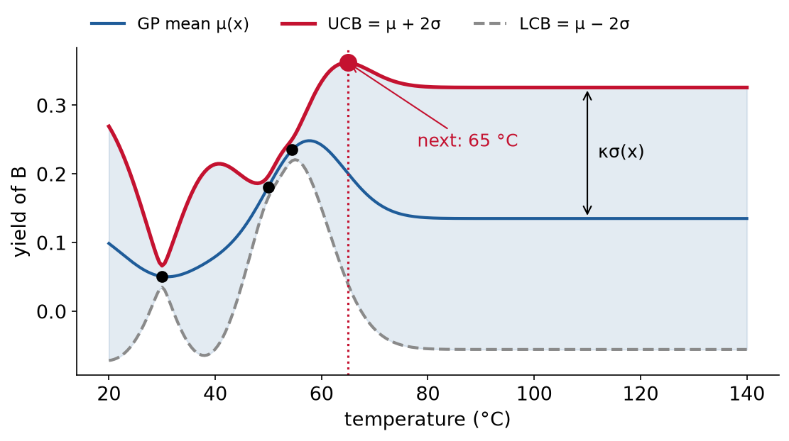
Fig. 118 UCB with \(\kappa = 2\) on the GP after three experiments. Its maximum, 65 °C, is the next experiment.

One GP, three choices

• After three experiments (30, 50 and 54 °C), the three acquisitions pick 56 (PI), 61 (EI) and 65 °C (UCB, \(\kappa = 2\)).

• PI stays closest to the incumbent; UCB with \(\kappa = 2\) reaches furthest into the unknown.

• Same data, same GP: the acquisition function alone sets the next experiment.

Donald Jones and EGO

Definition: efficient global optimization (EGO)

Efficient global optimization (EGO) fits a kriging model (a GP) to a space-filling set of samples, then samples where expected improvement is largest, refits, and repeats (Jones, Schonlau and Welch, 1998).

As the paper describes it:

• Start from a space-filling design, about 10 points per input.

• Fit the kriging model by maximum likelihood, and check it once by cross-validation.

• Loop: maximize EI; sample there; re-estimate the model.

• Stop when the expected improvement is less than 1% of the best current value.

• Kriging is the GP of geostatistics. It is named after Danie Krige, a South African mining engineer who estimated gold ore grades in the Witwatersrand mines from samples (NAE memorial tribute).

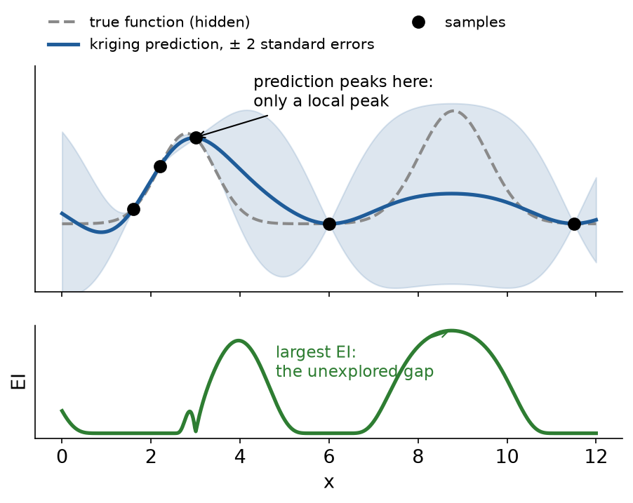
Fig. 119 The idea of the paper’s 1-D example, redrawn on a function of our own. The prediction alone peaks at a local peak near the cluster of samples; EI is largest in the unexplored gap.

Where the ideas come from

• Kushner (1964): probability of improvement, for “a multipeak curve in the presence of noise”.

• Šaltenis (1971), Močkus (1970s): expected improvement, and the Bayesian approach to seeking an extremum.

• Jones, Schonlau and Welch (1998): EGO, expected improvement on a kriging (GP) model. The paper that made BO standard in engineering design.

• Jones (2001): a taxonomy of response-surface methods for global optimization, and when each one fails.

• Snoek, Larochelle and Adams (2012): BO for tuning machine learning models, the start of its boom in machine learning.

Bayesian optimization in BoTorch

• BoTorch is a library for Bayesian optimization built on PyTorch, from Meta (Balandat et al., 2020).

• Its GPs come from GPyTorch.

• optimize_acqf maximizes the acquisition with L-BFGS-B (from SciPy), a gradient-based method. The gradients come from PyTorch’s automatic differentiation.

• Its UCB is UpperConfidenceBound(gp, beta), which computes \(\mu + \sqrt{\beta}\,\sigma\). So BoTorch’s beta is \(\kappa^2\): beta=4.0 is \(\kappa = 2\).

• Documentation and tutorials: botorch.org/docs.

The pieces of the worked example, in order:

• SingleTaskGP(T, y, input_transform=..., outcome_transform=...): the GP. Normalize maps the temperature to [0, 1]; Standardize gives the yields mean 0 and standard deviation 1. The kernel’s settings are then sensible defaults.

• ExactMarginalLogLikelihood and fit_gpytorch_mll: fit the GP’s settings (length scale, noise) by maximizing the marginal likelihood, as in Lecture 14.

• LogExpectedImprovement(gp, best_f=y.max()): the acquisition function, with the incumbent.

• optimize_acqf(acq, bounds, q=1, num_restarts=10, raw_samples=200): find the input that maximizes it. It scores 200 random candidates, starts 10 gradient-based searches from the best, and returns the winner. q=1: one experiment at a time.

for i in range(10):
    # 1. the surrogate: a GP fitted to every experiment so far
    gp = SingleTaskGP(
        T,
        y,
        input_transform=Normalize(d=1),
        outcome_transform=Standardize(m=1),
    )
    mll = ExactMarginalLogLikelihood(gp.likelihood, gp)
    fit_gpytorch_mll(mll)

    # 2. the acquisition: expected improvement over the best yield so far
    acq = LogExpectedImprovement(gp, best_f=y.max())

    # 3. the next experiment: where the acquisition is largest
    T_next, _ = optimize_acqf(
        acq,
        bounds=bounds,
        q=1,
        num_restarts=10,
        raw_samples=200,
    )

    # 4. run it, and add it to the data
    y_next = run_experiment(T_next)
    T = torch.cat([T, T_next])
    y = torch.cat([y, y_next])

• Optimizing the acquisition function is itself an optimization, but a cheap one: the GP is a formula, so gradient-based search works there. The expensive part, the experiment, happens once per pass.

A second knob: the time in the tank

• The feed pump sets the flow \(q\), so the time in the tank is \(\tau = V/q\), with \(V\) the volume of the tank. Now \(\tau\) is a knob too, from 1 to 30 min.

• Same loop, two inputs: Normalize(d=2) scales both temperature and \(\tau\) to [0, 1].

• The two knobs interact: with 30 minutes in the tank, the best temperature drops from 80 to 67 °C, and the best yield rises from 0.46 to 0.55.

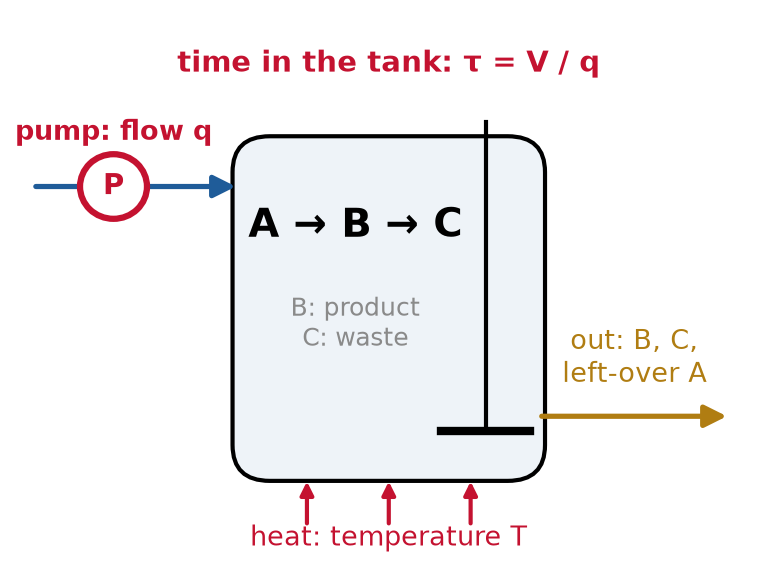
Fig. 120 The second knob. The pump sets the flow \(q\), and so the time in the tank \(\tau = V/q\).

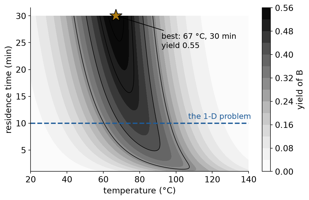
Fig. 121 The yield over both knobs. The 1-D problem is the dashed line; the best point (gold) needs the longest residence time and a lower temperature.

Comparing optimizers over several seeds

• One run proves nothing: BO is random (the noise, the random candidates). Report:

  • several seeds (here 10);

  • a baseline (random search, and two classic optimizers);

  • the best-so-far curve against experiments, with its spread;

  • the budget, counted.

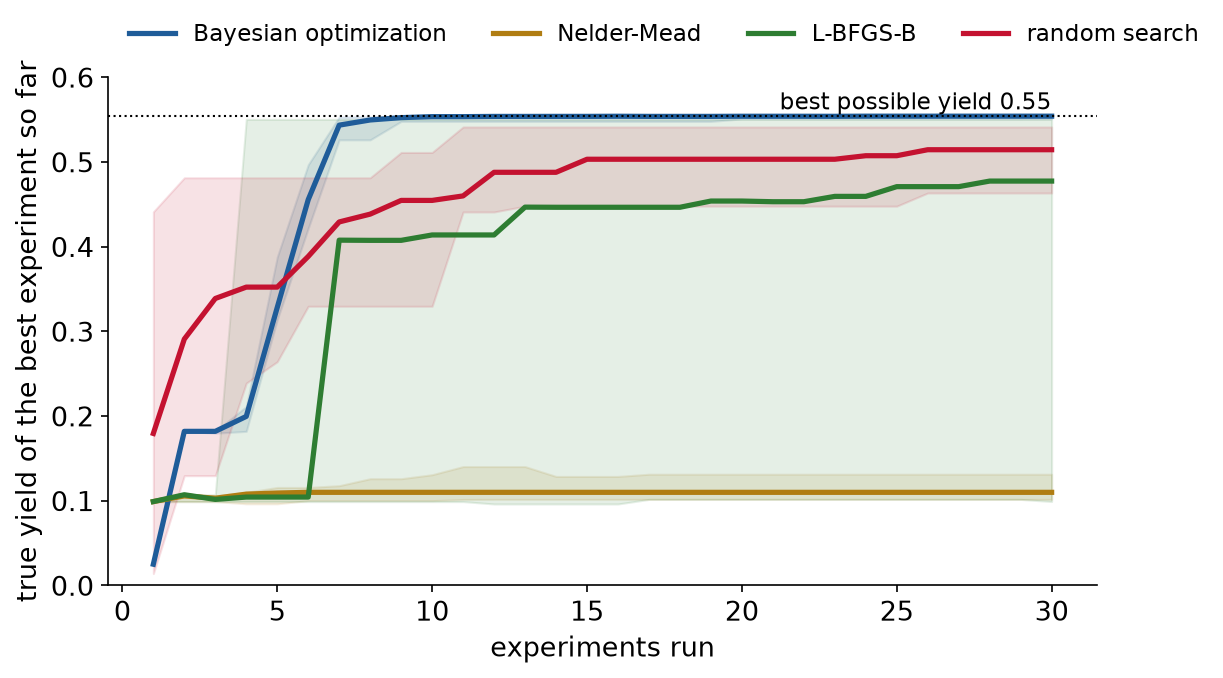
Fig. 122 Best-so-far over 10 seeds (median, with the range). BO reached 98% of the best possible yield in all 10 seeds, in 8 experiments (median).

Bayesian optimization against gradient-based optimization

Same reactor, same two knobs, same noise, 30 experiments, 10 seeds. Each method starts from the lab’s cold side:

Method	Reached 98% of the best yield	After 30 experiments (median)
Bayesian optimization (LogEI)	10 of 10 seeds, median 8 experiments	100%
L-BFGS-B, finite-difference gradients	2 of 10 seeds	86%
Nelder–Mead	0 of 10	20%
Random search	0 of 10	93%

• L-BFGS-B (a quasi-Newton method) estimates gradients by nudging each input. Each gradient costs experiments, and the measurement noise swamps the small differences in the flat, cold region. It often stops where it started.

  • At 40 °C and 10 min, its step of 1.2 °C changes the true yield by 0.008. The noise in the difference of two experiments has a standard deviation of 0.014, almost twice as large.

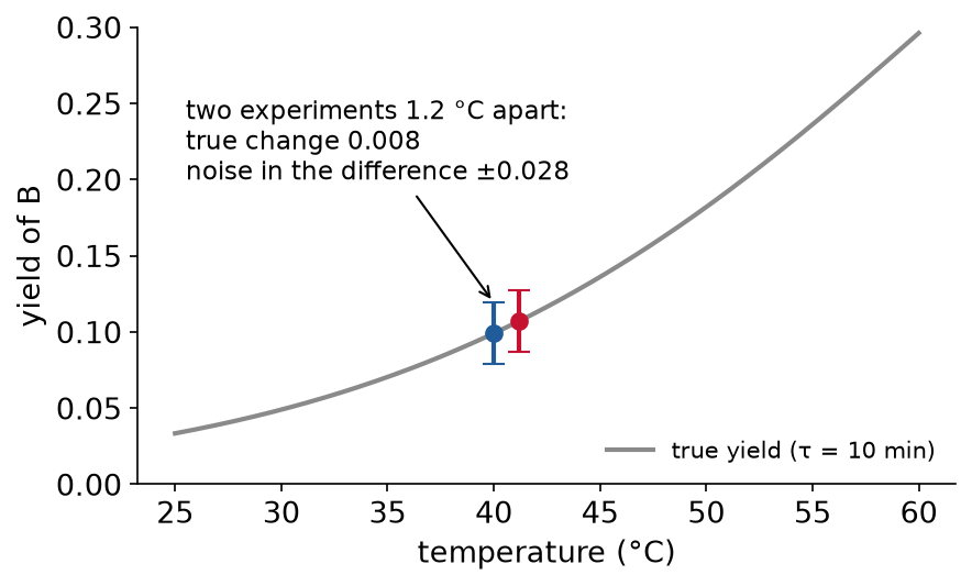
Fig. 123 A finite-difference gradient on the cold side. The change it tries to measure is smaller than the noise.

• Nelder–Mead (a simplex method) needs no gradients, but it is local and it stalls on the flat, noisy plateau.

• Random search never gets stuck, but it never focuses either.

When to use which:

• Gradient-based (Newton, L-BFGS, IPOPT): cheap evaluations, smooth functions, gradients available (from a model, by automatic differentiation or adjoints), and many variables, up to millions. It finds a local optimum fast.

• Bayesian optimization: expensive evaluations (minutes to weeks), no gradients, noise, a budget of tens to hundreds, and few inputs (up to about 20). It explores the whole range, but with no guarantee of finding the global optimum. Its overhead, seconds per step, is small compared with an experiment.

• Other derivative-free methods (Nelder–Mead, evolutionary algorithms): no gradients, but enough budget for hundreds or thousands of evaluations.

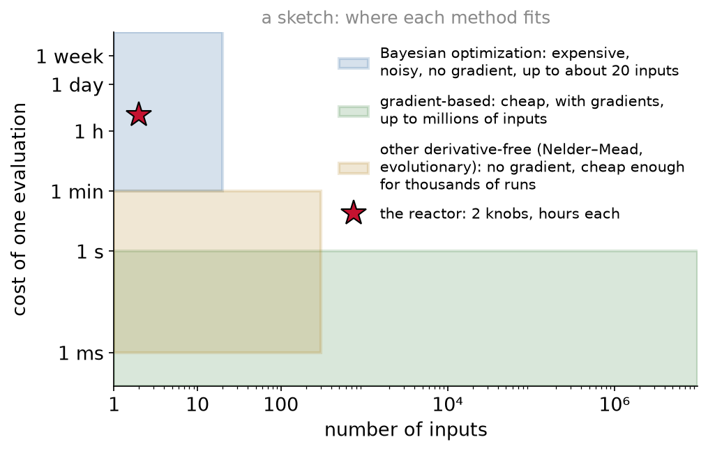
Fig. 124 A sketch of where each kind of optimizer fits. The reactor (red star) has two knobs and hours per experiment.

Where Bayesian optimization is used

• Chemical synthesis. Shields et al. (2021) had 50 expert chemists and engineers play a reaction optimization game against BO. BO needed fewer experiments on average, and was more consistent.

• Self-driving laboratories. A mobile robotic chemist (Burger et al., 2020) ran 688 experiments over eight days, in a space of ten variables, with batched BO choosing them. It found a photocatalyst six times more active than the starting formulations.

• Batteries. Attia et al. (2020) combined BO with early predictions of battery life, and ranked 224 fast-charging protocols in 16 days. Exhaustive testing without early prediction would have taken over 500 days.

• Process design. Kriging surrogates, the GPs of engineering, choose which flowsheet simulations to run when each one is expensive (Caballero and Grossmann, 2008).

• Engineering design. Wing shapes and other designs evaluated by expensive simulations (Forrester, Sóbester and Keane, 2008).

• Machine learning. Choosing a model’s settings, such as the learning rate, when each training run takes hours (Snoek et al., 2012). BO tuned the settings of the Go program AlphaGo before its 2016 match, where each test is many games: its win rate against its old self rose from 50% to 66.5% (Chen et al., 2018).

• Control. Tuning the controller of an automotive throttle valve on the real test bench: as good as or better than hand tuning, in about ten experiments (Neumann-Brosig et al., 2020).

• Online experiments. Facebook tuned the settings of a ranking system and of its server software (compiler flags). Each try is a live test with noisy results (Letham et al., 2019).

• Food. Google tuned a chocolate chip cookie recipe (sugar, salt, vanilla, chips) by taste tests, over 144 experiments (Solnik et al., 2017).

Extensions engineers need

All four are in BoTorch:

• Constraints: the best yield may need a temperature the reactor cannot take. A second GP learns that limit (the temperature of a hot spot, say) from the same experiments, and the acquisition is multiplied by the probability of respecting it, so BO proposes only runs likely to stay within the limit.

• Batches: the lab has four reactors. Choose four experiments at once (q=4, with a batch acquisition such as qLogEI).

• Several objectives: yield and cost, or yield and energy. BO maps the Pareto front, the set of best trade-offs (qEHVI, expected hypervolume improvement).

• Several fidelities: a cheap, rough simulation and an expensive, exact one. BO decides which to run, and where.

Limitations and trade-offs

• Dimension. BO works best up to about 20 inputs. Beyond that the GP needs far more data to be useful.

• Cost of the GP. Fitting grows as \(n^3\) with the number of evaluations \(n\). Fine for hundreds, slow for many thousands. With thousands of cheap evaluations, use something else.

• The prior matters. The kernel assumes a smoothness. A function with jumps or cliffs breaks it, and the band is then wrong.

• Cold start. With two or three points the GP’s uncertainty is not trustworthy yet. Seed the loop with a small, spread-out set of experiments.

• Noise and the incumbent. With noisy measurements, the best measured value is partly luck (the reactor’s best measured yield, 0.474, had a true yield of 0.461). Report the model’s best, or repeat the best experiment.

• One run is not evidence. BO is random. Use several seeds and a baseline.

Active learning: the same loop, a different goal

Definition: active learning

Active learning chooses each next experiment to make the model good everywhere, usually where it is most uncertain: \(x_{n+1} = \arg\max_x \sigma(x)\).

• \(x_{n+1} = \arg\max_x \sigma(x)\) reads: the next experiment is the input where the GP’s uncertainty \(\sigma(x)\) is largest, the widest point of the band.

• Same GP, same loop. Only the acquisition function changes: the goal is a model, not one optimum.

• On the reactor, from the same two old runs, six more experiments each: BO (EI) crowds around 80 °C; active learning spreads from 20 to 140 °C and leaves a narrow band everywhere.

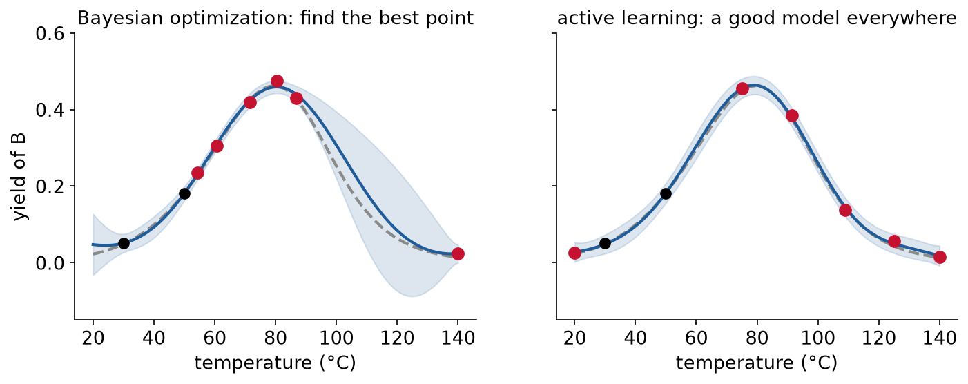
Fig. 125 Six more experiments each, from the same two old runs (black). Left: chosen by expected improvement. Right: chosen where the GP is most uncertain.

In-class demo

• l15-bayesian-optimization.ipynb: BoTorch on the reactor. One knob (temperature) from two old runs, the loop printed experiment by experiment, and the answer checked against the true curve. Then two knobs (temperature and residence time), against random search over five seeds.

Summary

Bayesian optimization is for objectives that are expensive, noisy and without gradients, when the budget is tens of evaluations. It fits a Gaussian process to every evaluation so far, and an acquisition function turns the GP’s mean and uncertainty into the next experiment, balancing exploitation (go where it looks good) against exploration (go where it is unsure). PI, EI and UCB are three recipes for that balance; LogEI is the numerically safe EI that BoTorch uses. Gradient-based methods need cheap, noise-free evaluations; when each evaluation is an experiment, BO spends the budget where it can still learn or gain.

Resources

• Frazier, A Tutorial on Bayesian Optimization. The loop, the acquisition functions and the extensions, in one readable tutorial.

• Garnett, Bayesian Optimization. The textbook, free online.

• Shahriari et al. (2016), Taking the Human Out of the Loop. The standard review (author’s copy).

• Jones, Schonlau and Welch (1998), Efficient Global Optimization of Expensive Black-Box Functions. EGO: expected improvement on a GP, the paper that made BO standard in engineering design (published version, on Welch’s page).

• Jones (2001), A Taxonomy of Global Optimization Methods Based on Response Surfaces. Which surrogate-based methods work, which can fail, and why (mirror copy).

• BoTorch tutorials. Worked examples of every piece used today, and of the extensions.

• Shields et al. (2021), Bayesian reaction optimization as a tool for chemical synthesis. BO against 50 expert chemists and engineers (author lab’s copy of the published paper).

Assignment

Assignment 5, four models of a bioreactor, is released today and due Wednesday 10-28.

Practice module

Practice module for this session, for participation credit.