Lecture 13: Scientific machine learning: PINNs, neural ODEs and neural DAEs

At a glance

• Session Lecture 13, Week 7

• Arc Machine learning and deep learning

• Slides Deck for this session

• Practice Practice module for this session

• Worked examples l13-pinn-jax.ipynb, a physics-informed network built from scratch in JAX; l13-neural-dae.ipynb, a fed-batch bioreactor as a neural ODE in Diffrax and as a neural DAE in SiNDAE

• Tools JAX and Optax for the PINN; Diffrax and Equinox for the neural ODE; SiNDAE, Pyomo and the POUNCE solver for the neural DAE

Why this matters

A fed-batch bioreactor

A fed-batch bioreactor starts with cells and a growth medium. Substrate (the cells’ food, such as glucose) is fed during the run, and nothing is taken out until harvest.

• The volume grows with the feed.

• The feed sets how much substrate the cells see, so it steers growth and product formation.

• It is used to make monoclonal antibodies (mAbs) and other therapeutic proteins, recombinant proteins in E. coli, baker’s yeast and penicillin (summary).

• Fed-batch is still “the most commonly utilized process type for biomanufacturing” (Bioprocess and Biosystems Engineering, 2024).

• Chinese hamster ovary (CHO) cells make about 80% of U.S.-licensed mAb products (mAbs, 2025).

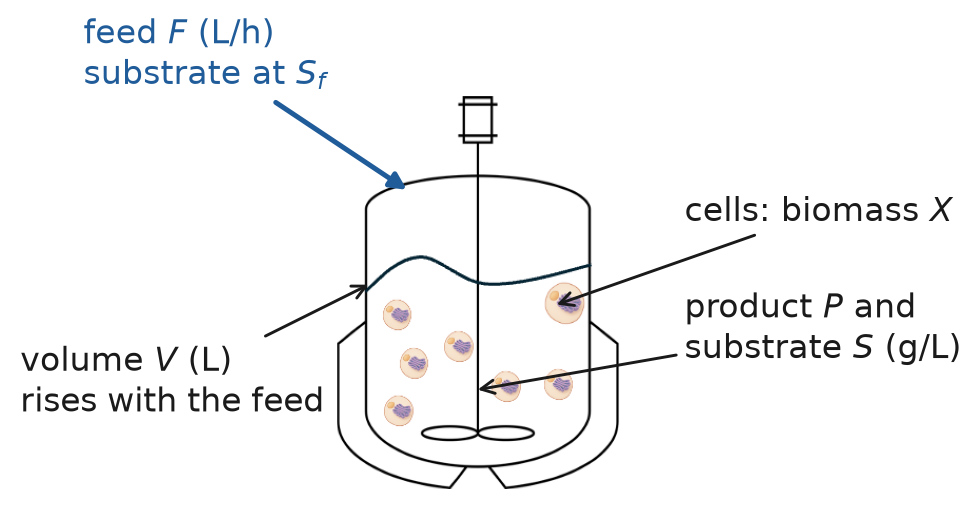
Fig. 75 The fed-batch bioreactor and its four states.

The model has four states: biomass \(X\), product \(P\), substrate \(S\) (all in g/L) and volume \(V\) (L). Each balance reads accumulation = what comes in − what leaves + what is made − what is used:

\[ \underbrace{\frac{dX}{dt}}_{\text{accumulation}} = \underbrace{\mu\,X}_{\text{growth}} - \underbrace{\frac{F}{V}\,X}_{\text{dilution by the feed}} \]

\[ \frac{dP}{dt} = \underbrace{Y_{P/X}\,\mu\,X}_{\text{made by growing cells}} - \underbrace{\frac{F}{V}\,P}_{\text{dilution}} \]

\[ \frac{dS}{dt} = \underbrace{\frac{F}{V}\,(S_f - S)}_{\text{fed in}} - \underbrace{\frac{\mu\,X}{Y_{X/S}}}_{\text{eaten by the cells}} \]

\[ \frac{dV}{dt} = \underbrace{F}_{\text{feed rate}} \]

• \(F\) is the feed rate (L/h) and \(S_f\) the substrate concentration in the feed (g/L).

• \(Y_{P/X}\) and \(Y_{X/S}\) are yields: grams of product per gram of cells, and grams of cells per gram of substrate.

• \(\mu\) is the specific growth rate (1/h): the kinetics. Every other term is bookkeeping. \(\mu\) is the part we do not know.

Why learn the kinetics

• The balances are conservation of mass: they are certain.

• The rate laws are not. They depend on the strain, the medium and the conditions, and a cell is a large reaction network. Even a simplified CHO network has 30 reaction rates, \(v_1\) to \(v_{30}\), each with its own law and parameters.

• In a monoclonal antibody process the scales stack up: the reactor, the cell, and the Golgi apparatus where the antibody is finished.

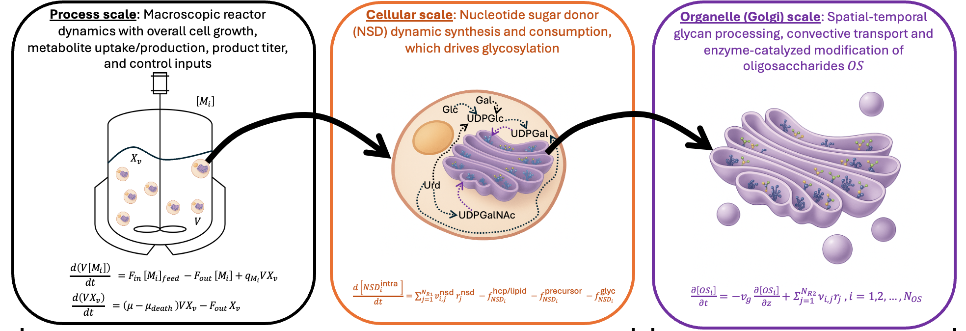
Fig. 76 A monoclonal antibody process across three scales: reactor, cell, and Golgi apparatus.

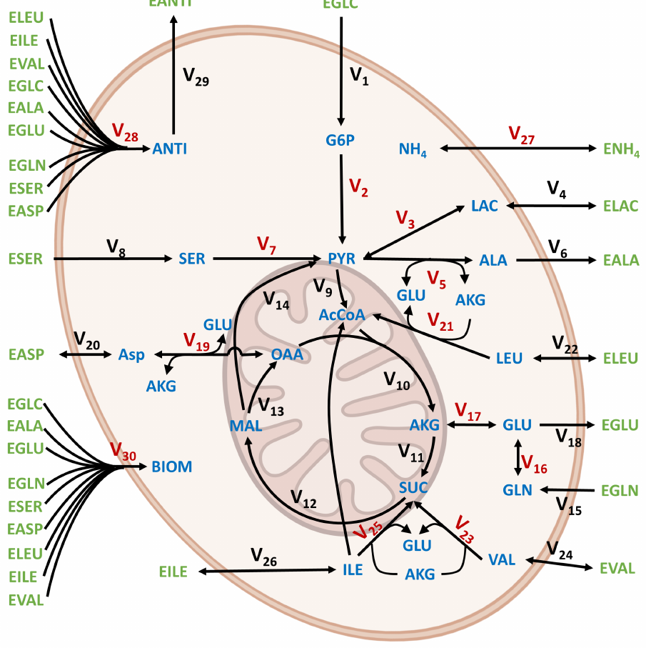
Fig. 77 A simplified CHO metabolic network with 30 reaction rates. Fig. 5 of Wang, Harcum and Xie (2025), CC BY 4.0.

So we keep the balances and let a network learn \(\mu\) from data. Here we use three batches.

Inference on unseen data

Three models learn from the same three training batches, 0 to 40 h. Then each predicts a new batch, with a different starting charge, for 60 h.

• Purely data-driven: a network for the whole right-hand side, \(dx/dt = \mathrm{NN}(x)\). No physics.

• Physics-informed: the balances, with only \(\mu\) learned.

• Physics-enforced: the same balances as a neural DAE, with \(S \ge 0\) as a constraint.

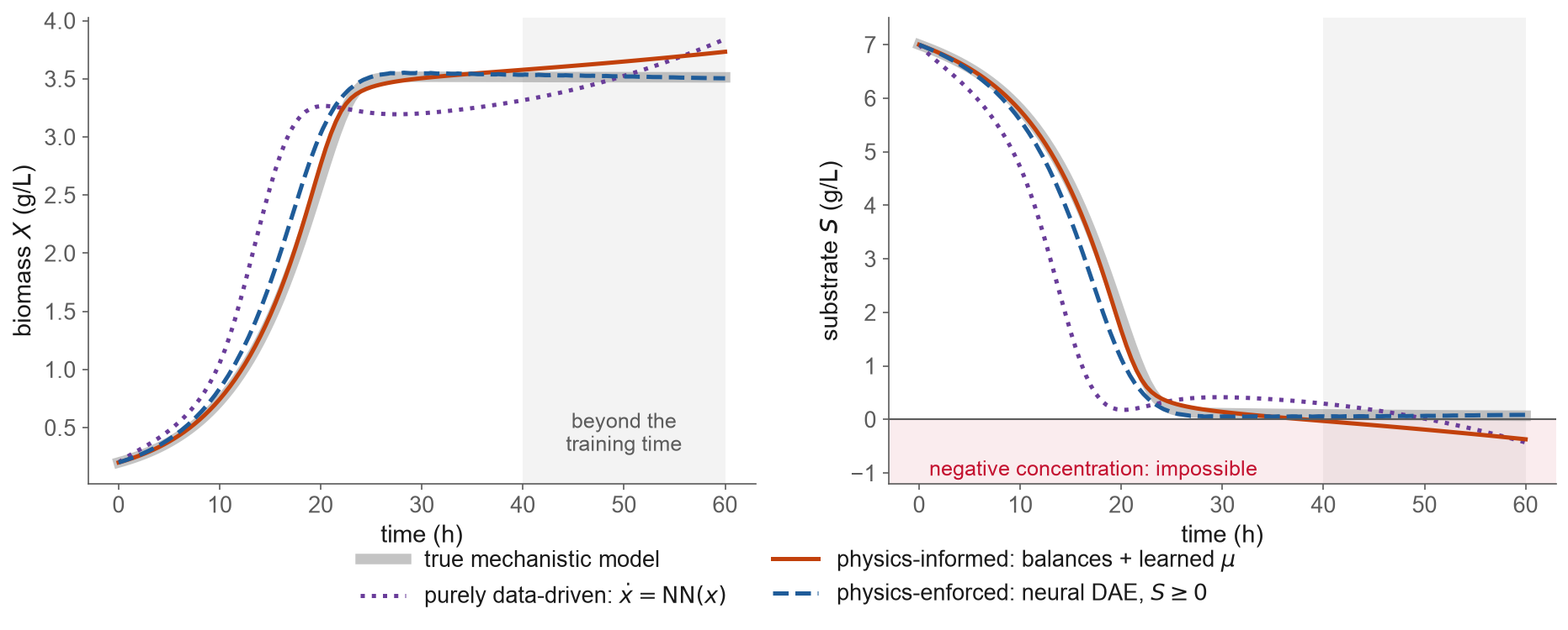
Fig. 78 The new batch: the true mechanistic model and three learned models.

New batch, 60 h	Lowest substrate	Hours with \(S < 0\)	Biomass error (RMSE)
Purely data-driven	−0.43 g/L	10	0.43 g/L
Physics-informed	−0.37 g/L	22	0.09 g/L
Physics-enforced (neural DAE)	0.05 g/L	0	0.15 g/L
True mechanistic model	0.07 g/L	0

• The data-driven model knows nothing about the balances, and it extrapolates worst.

• The balances help, but a negative concentration is still possible: nothing in the model forbids it.

This session is about how to put physics into a learned model so that this cannot happen.

Gen 0 to Gen 2

Machine learning in science and engineering has come in generations.

• Gen 0, surrogate models. “Often, the codes are computationally expensive to run, and a common objective of an experiment is to fit a cheaper predictor of the output to the data” (Sacks et al., 1989). A surrogate is a cheap stand-in for an expensive model.

• Gen 1, machine learning with intention. The surrogate also says how uncertain it is, and the uncertainty decides where to sample next (Jones, Schonlau and Welch, 1998). This is the idea behind Bayesian optimization: a cheap surrogate with its uncertainty chooses the next expensive experiment or simulation.

• Neither generation knows any physics. Everything comes from the data.

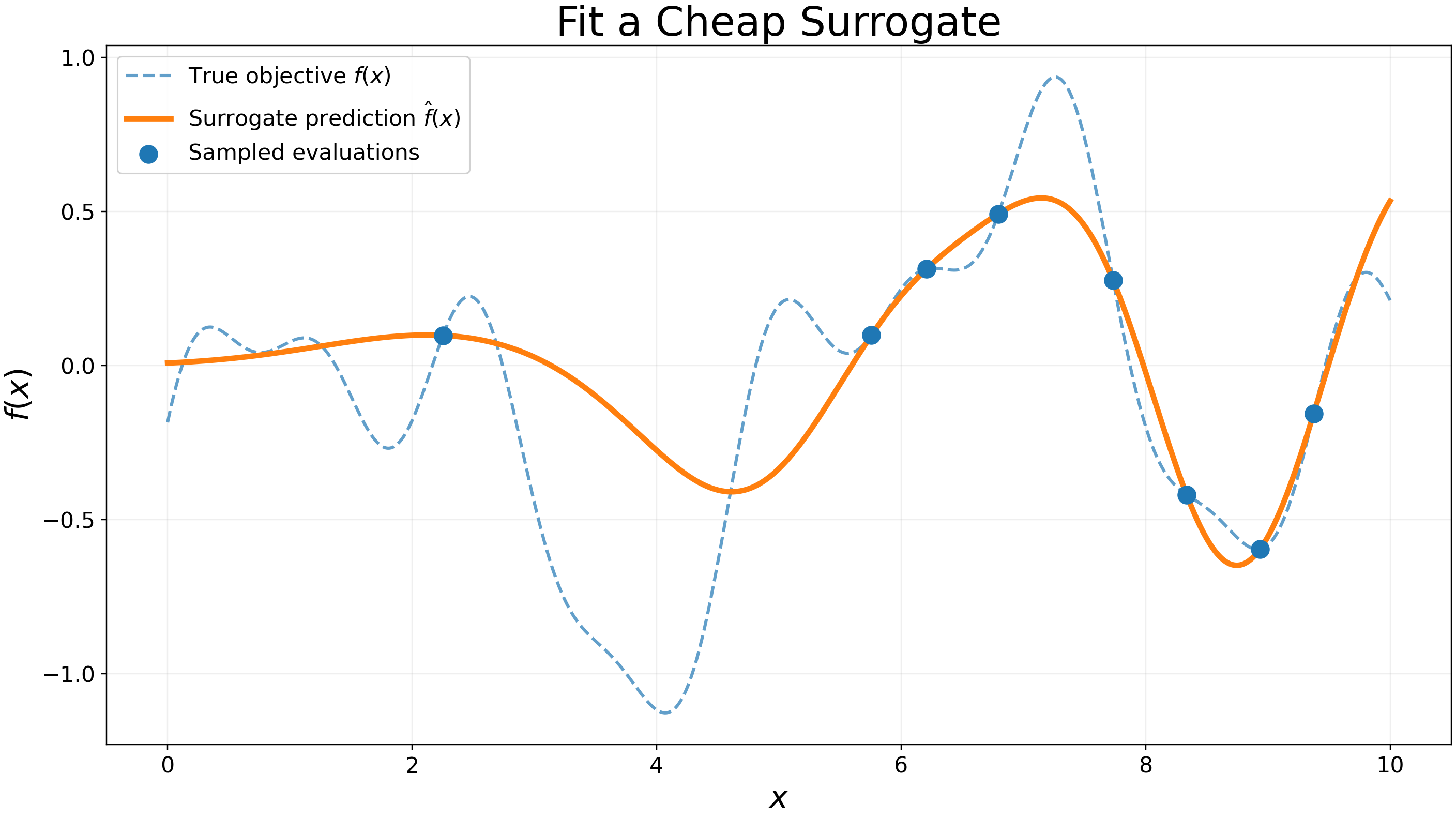
Fig. 79 Gen 0: a cheap surrogate fitted to a few evaluations of an expensive function.

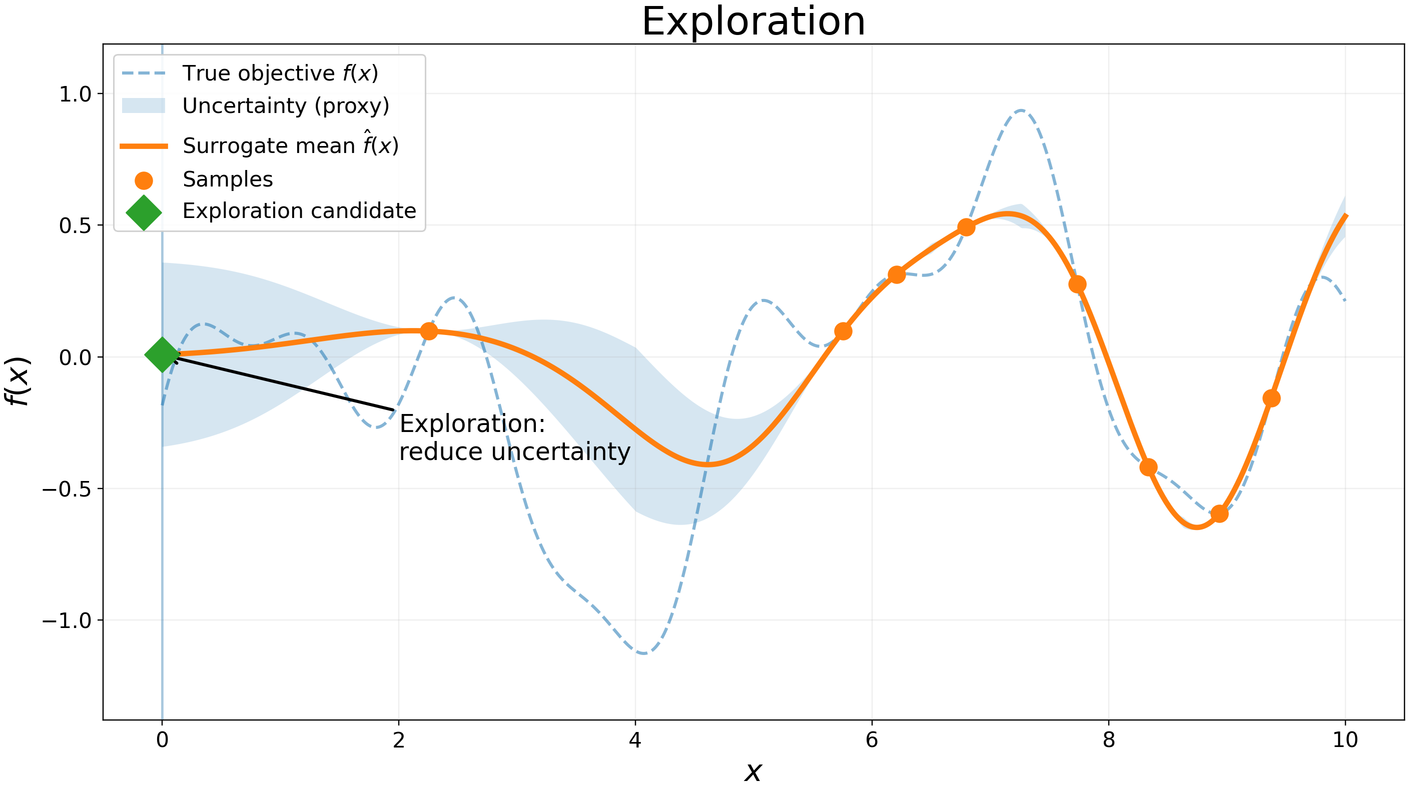
Fig. 80 Gen 1: the surrogate’s uncertainty (shaded) chooses the next sample.

Gen 2 keeps the mechanistic model and adds machine learning only where the physics is unknown.

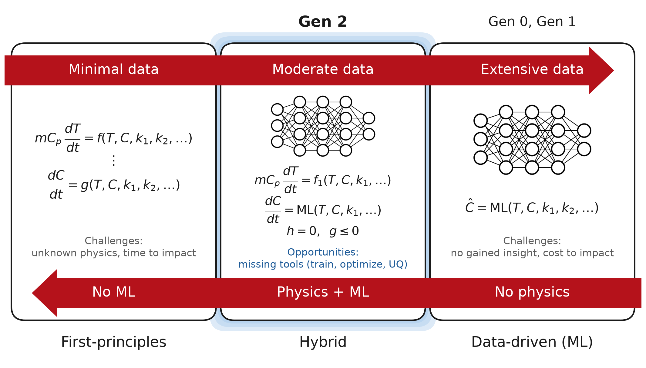
Fig. 81 First-principles, hybrid and data-driven models, after Fig. 1 of Shah et al. (2025).

Definition: scientific machine learning (SciML)

Scientific machine learning combines mechanistic, first-principles models (balances, rate laws, constraints) with machine learning, so the network learns only what the physics does not already say.

The pattern is the same across engineering and physics: conservation laws are known, and one closure term is not.

\[ mL\ddot\theta = -mg\sin\theta - \underbrace{F_f(\dot\theta)}_{\text{friction}} \qquad \rho c_p\frac{\partial T}{\partial t} = \kappa\frac{\partial^2 T}{\partial z^2} + \underbrace{q(T)}_{\text{heat source}} \]

\[ \frac{dC}{dt} = \frac{q}{V}(C_f - C) - \underbrace{r(C, T)}_{\text{kinetics}} \qquad A\frac{dh}{dt} = q_\text{in} - \underbrace{q_\text{out}(h)}_{\text{valve law}} \]

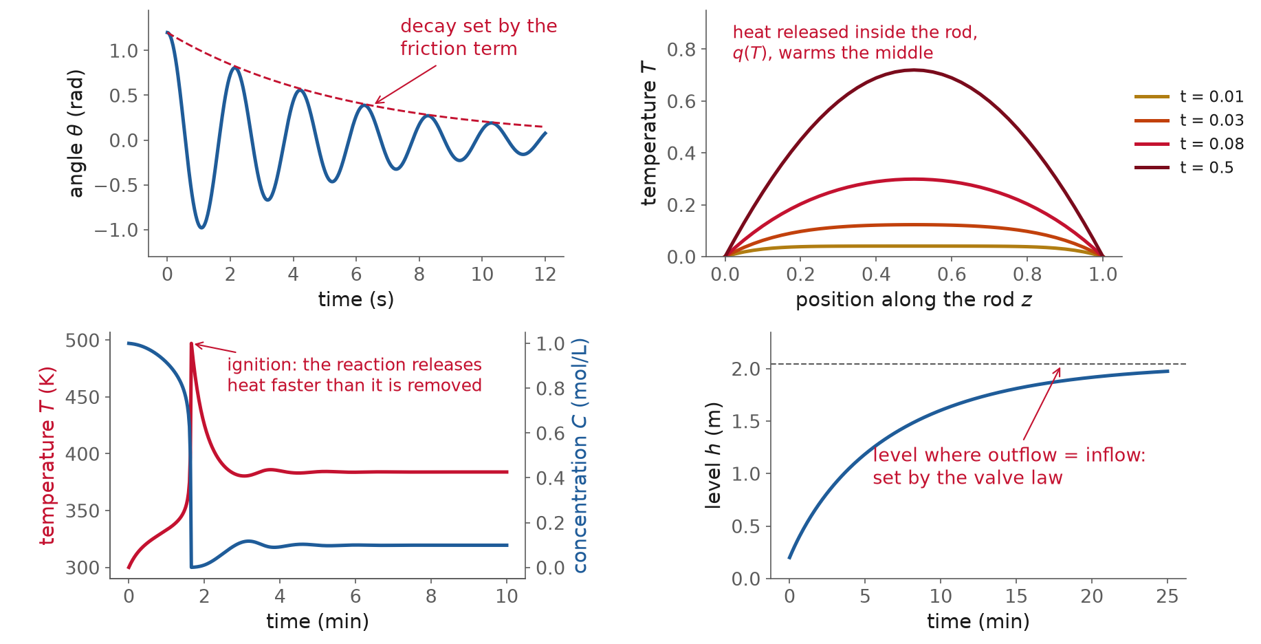
Fig. 82 A pendulum, heat conduction in a rod, an exothermic CSTR (continuous stirred-tank reactor), and a tank. In each, the underbraced term is a candidate for a network.

There are four ways to add the physics to a network. Each one guarantees something different.

	Where the physics lives	High-level formulation
PINN	the loss	\(L = L_\text{data} + \lambda\,L_\text{physics}\)
Neural ODE	the right-hand side of the ODE	\(\dfrac{dx}{dt} = f\big(x, \mathrm{NN}(x;\theta)\big)\)
Neural DAE	the constraints of one optimization problem	\(\min_\theta L_\text{data}\) s.t. \(\dot x = f,\ h = 0,\ g \le 0\)
Projection layer	the last layer of the network	\(y = P_{\{Ay = b\}}\big(\mathrm{NN}(u;\theta)\big)\)

Learning objectives

By the end of this session you should be able to:

• Explain what a physics-informed neural network (PINN) minimizes, and why its physics holds only approximately.

• Build a PINN in JAX and compare its extrapolation with a plain network.

• Derive a neural ODE from a recurrent network by letting the time step go to zero, and train one with a differentiable ODE solver.

• Explain why some physics must be enforced rather than penalized, and what makes a model a differential-algebraic equation (DAE).

• Contrast the sequential and simultaneous approaches to training a dynamic model.

• Train a neural DAE with SiNDAE, and check that its predictions satisfy the constraints.

• Compare PINNs, neural ODEs, neural DAEs and projection layers: where the physics lives, and what each one guarantees.

Physics-informed neural networks (PINNs)

The example: a damped spring-mass

A mass hangs from a spring, with a damper beside it. A car’s suspension is the same system. Drag the mass, let go, and change \(m\), \(\mu\) and \(k\):

The equation of motion comes from Newton’s second law: mass times acceleration equals the sum of the forces.

\[ m\,x'' = F_\text{spring} + F_\text{damper} \]

• The spring pulls back toward rest (Hooke’s law): \(F_\text{spring} = -k\,x\).

• The damper opposes the motion (viscous friction): \(F_\text{damper} = -\mu\,x'\).

• Move both forces to the left:

\[ \underbrace{m\,x''}_{\text{inertia}} + \underbrace{\mu\,x'}_{\text{damper force}} + \underbrace{k\,x}_{\text{spring force}} = 0, \qquad x(0) = 1\ \text{m}, \quad x'(0) = 0 \]

Symbol	Meaning	Value here
\(x\)	displacement from rest, up is positive (m)
\(x' = dx/dt\)	velocity (m/s)
\(x'' = d^2x/dt^2\)	acceleration (m/s²)
\(m\)	mass (kg)	1
\(\mu\)	damping coefficient (N·s/m)	4
\(k\)	spring stiffness (N/m)	400

Gravity only shifts the rest position, so measuring \(x\) from rest removes it.

The task.

• We measure \(x\) at 10 times, all in the first 0.36 s: about one oscillation.

• We want \(x(t)\) over the whole second. From 0.36 s to 1 s there are no measurements.

• We know the equation of motion and the values of \(m\), \(\mu\) and \(k\).

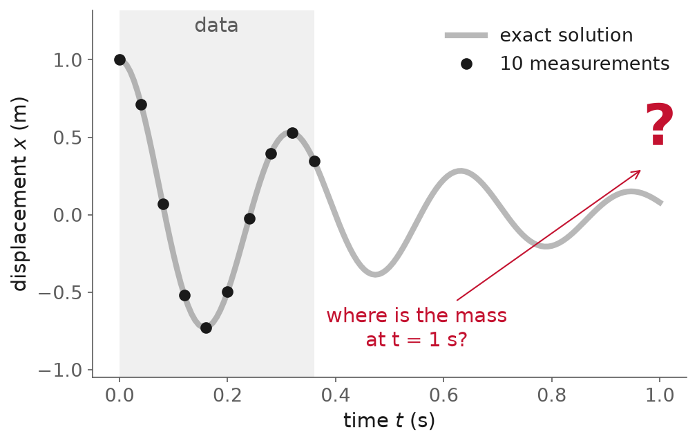
Fig. 83 Ten measurements, all inside the gray band. Everything to its right is extrapolation.

A plain network

• A network \(x_\text{NN}(t;\theta)\) takes the time \(t\) and returns the displacement.

• It is trained on the data alone, by minimizing the mean squared error over the \(N = 10\) points:

\[ L_\text{data}(\theta) = \frac{1}{N}\sum_{i=1}^{N} \big(x_\text{NN}(t_i;\theta) - x_i\big)^2 \]

• It fits the 10 points. After the last one it has nothing to go on, and drifts to a flat line.

Physics in the loss

Definition: physics-informed neural network (PINN)

A PINN is a network trained to fit the data and, at the same time, to make the residual of the governing equation small.

Raissi, Perdikaris and Karniadakis introduced them as “neural networks that are trained to solve supervised learning tasks while respecting any given law of physics described by general nonlinear partial differential equations” (2019). For the spring-mass the loss is

\[ L(\theta) = \underbrace{\frac{1}{N}\sum_{i=1}^{N} \big(x_\text{NN}(t_i) - x_i\big)^2}_{\text{data loss}} \; + \; \lambda\, \underbrace{\frac{1}{M}\sum_{j=1}^{M} \Big(m\,x_\text{NN}''(t_j) + \mu\,x_\text{NN}'(t_j) + k\,x_\text{NN}(t_j)\Big)^2}_{\text{physics loss}} \]

• The second term is the residual of the equation: zero for a function that obeys it exactly.

• \(\lambda\) weighs the physics against the data. We use \(\lambda = 10^{-4}\): the residual is in newtons, hundreds of times larger than the displacement in meters, so its weight is small.

• The derivatives \(x_\text{NN}'\) and \(x_\text{NN}''\) come from automatic differentiation (Lecture 11): differentiate the network with respect to its input \(t\).

Definition: collocation point

A collocation point is a time at which we ask the equation to hold. It needs no measurement, so we can place as many as we like, anywhere.

Here there are \(M = 40\) collocation points, spread over the whole interval from 0 to 1 s, where we have no data.

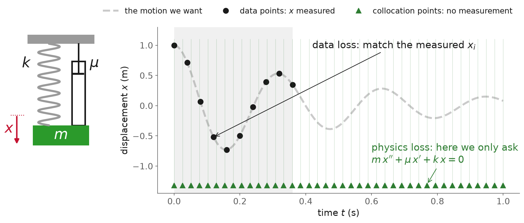
Fig. 84 Data points (black) feed the data loss. Collocation points (green) feed the physics loss.

Physics is favored, not enforced. The optimizer makes the residual small, not zero.

A PINN in JAX

JAX is a Python library for numerical computing that can differentiate any function you write in it (docs). Optax is a library of optimizers for JAX, Adam among them (docs).

The network: one (W, b) pair per layer, three hidden layers of 32 tanh units. tanh is smooth, so its second derivative exists.

• W starts random, scaled by \(1/\sqrt{n_\text{in}}\) (the number of inputs), a standard choice that keeps tanh from saturating at the start (LeCun et al., 1998).

def init(key, sizes):
    params = []
    for n_in, n_out in zip(sizes[:-1], sizes[1:]):
        key, sub = jax.random.split(key)
        W = jax.random.normal(sub, (n_in, n_out)) * np.sqrt(1 / n_in)
        params.append((W, jnp.zeros(n_out)))
    return params

def net(params, t):
    h = t[:, None]
    for W, b in params[:-1]:
        h = jnp.tanh(h @ W + b)
    W, b = params[-1]
    return (h @ W + b)[:, 0]

def x_nn(params, t):
    return net(params, jnp.array([t]))[0]

The physics. jax.grad(f, argnums=1) returns the derivative of f with respect to its second argument, the time; applying it twice gives the second derivative. jax.vmap evaluates a function of one time at many times at once.

dx = jax.grad(x_nn, argnums=1)      # dx/dt
ddx = jax.grad(dx, argnums=1)       # d2x/dt2

def residual(params, ts):
    x = jax.vmap(lambda t: x_nn(params, t))(ts)
    v = jax.vmap(lambda t: dx(params, t))(ts)
    a = jax.vmap(lambda t: ddx(params, t))(ts)
    return m * a + mu * v + k * x

def data_loss(params):
    return jnp.mean((net(params, jnp.array(t_data)) - x_data) ** 2)

def physics_loss(params):
    return jnp.mean(residual(params, jnp.array(t_phys)) ** 2)

lam = 1e-4

def pinn_loss(params):
    return data_loss(params) + lam * physics_loss(params)

Training: optax.adam(1e-3) is Adam with learning rate 0.001; jax.jit compiles one step. Both networks start from the same weights and get the same steps. Only the loss differs.

def train(loss, steps=30_000):
    opt = optax.adam(1e-3)
    params = params0
    state = opt.init(params)

    @jax.jit
    def step(params, state):
        grads = jax.grad(loss)(params)
        updates, state = opt.update(grads, state, params)
        return optax.apply_updates(params, updates), state

    for _ in range(steps):
        params, state = step(params, state)
    return params

p_nn = train(data_loss)
p_pinn = train(pinn_loss)

Training and the result

Press Play: the two networks train, and then the three masses move with what each model predicts.

• For the first 1,000 steps both networks fit the 10 points, and both are wrong after 0.36 s (error over the whole second about 0.36 m).

• Between steps 1,300 and 8,500 the physics term pulls the PINN onto the oscillation: its error over the second falls from 0.34 m to 0.01 m.

• The plain network never improves after the data, at about 0.45 m.

• The PINN’s residual at the collocation points falls from 109 N to 0.7 N.

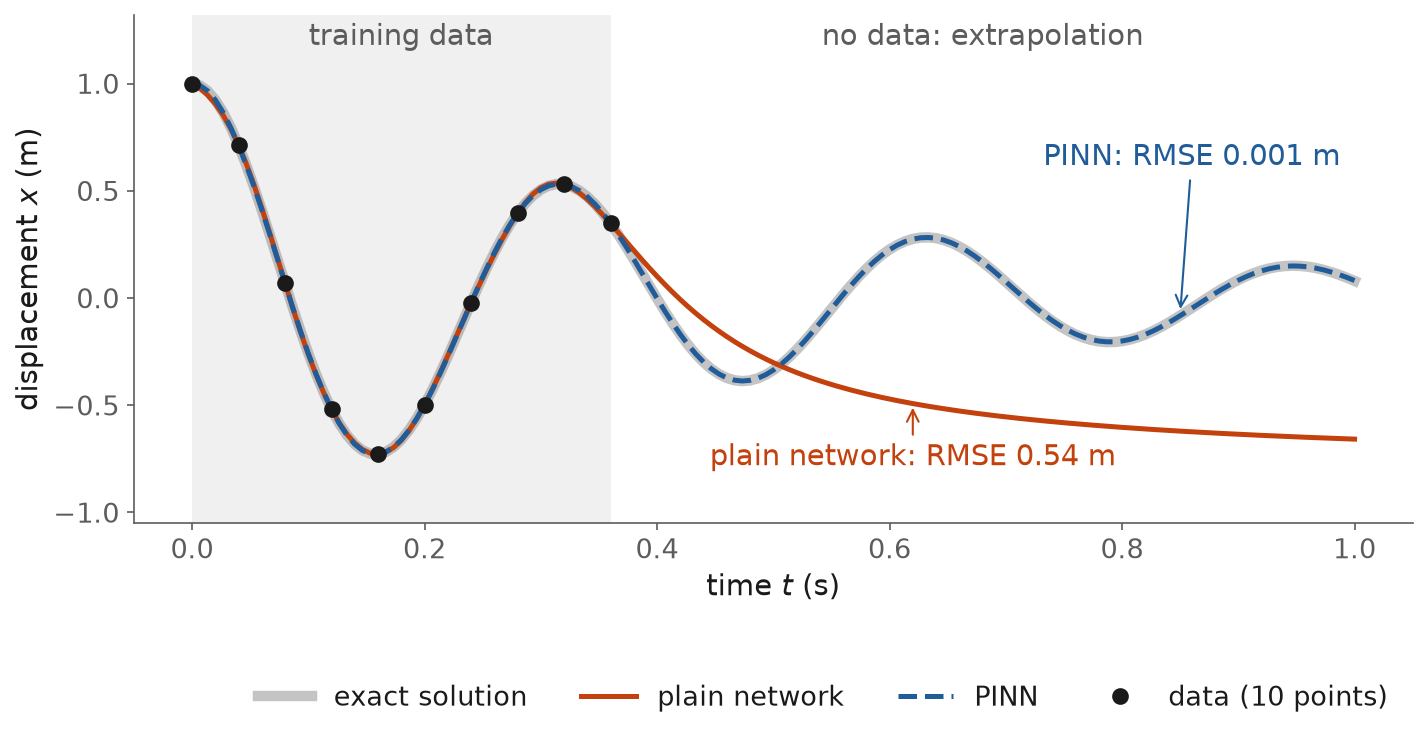
Fig. 85 After 30,000 steps. RMSE is the root mean squared error against the exact solution, after the last data point.

After 30,000 steps	Plain network	PINN
RMSE inside the data window	0.007 m	0.001 m
RMSE after the data (0.36 to 1 s)	0.54 m	0.001 m
Residual of the equation (RMS over 0 to 1 s)	163 N	5.3 N

• Inside the data window both are good.

• After it, the plain network is wrong by about half a meter. The PINN is right, because the equation told it what happens next.

• Ben Moseley’s blog post shows the same experiment.

The physics is a penalty, not a constraint

• After training, the PINN’s residual is 5.3 N (root mean square over the whole second). The forces in the equation reach 400 N, so it is small. It is not zero.

• At the 40 collocation points it is 0.7 N; between them it is larger. The physics is penalized only where you evaluate it.

• This is a soft constraint: the optimizer trades a little physics for a little data fit, with \(\lambda\) setting the exchange rate. Change \(\lambda\) and you get a different model.

Three known difficulties:

• Training can fail. Krishnapriyan and colleagues found that PINNs “can easily fail to learn relevant physical phenomena for even slightly more complex problems”, and that the cause is that “the PINN’s setup makes the loss landscape very hard to optimize” (NeurIPS 2021).

• The two loss terms compete. Wang, Teng and Perdikaris traced one failure to “an unstable imbalance in the magnitude of the back-propagated gradients” between the terms (2021).

• One trained PINN is one solution. The network learned the trajectory \(x(t)\) for this release from 1 m, with these \(m\), \(\mu\) and \(k\). Release the mass from 0.5 m, or change \(k\), and you must train again: the network learned a trajectory, not the law of motion. The way around it is to make the conditions inputs of the network, as physics-informed DeepONets do (Wang, Wang and Perdikaris, 2021).

From recurrent networks to neural ODEs

A PINN learns one solution. Here we learn the dynamics: the right-hand side of the differential equation, which works for any starting point.

The residual update

Residual networks and recurrent networks build a long computation from many small updates of a hidden state \(h\) (Chen et al., Eq. 1):

\[ h_{t+1} = h_t + f(h_t, \theta_t) \]

A recurrent neural network (RNN), from Lecture 12, applied over time uses the same \(f\) at every step, with steps of a fixed size \(\Delta t\):

\[ h_{k+1} = h_k + \Delta t\, f(h_k;\theta) \]

• For the spring-mass, the state is \(h = (x, v)\), position and velocity.

• The network learns how the state jumps from one sample to the next.

• This is the forward Euler method: new state = old state + step size × slope at the old state.

Chen, Rubanova, Bettencourt and Duvenaud: “These iterative updates can be seen as an Euler discretization of a continuous transformation” (Neural Ordinary Differential Equations, 2018).

Two pictures of the same idea:

• Recurrent network: \(h_0 \to h_1 \to h_2 \to \dots\), one jump of fixed size \(\Delta t\) at a time, with the same network \(f\) and the same weights \(\theta\) at every step.

• Neural ODE: \(h(t_0) \to\) an ODE solver for \(dh/dt = f(h, t;\theta) \to h(t)\) at any time. The network learns the arrows \(f\); the solver takes as many steps as it needs.

The limit

Read the hidden state as a function of time: \(h_k = h(t_k)\), with \(t_{k+1} = t_k + \Delta t\). The recurrent update, divided by the step:

\[ \frac{h(t_k + \Delta t) - h(t_k)}{\Delta t} = f\big(h(t_k), t_k, \theta\big) \]

Let \(\Delta t \to 0\). The left side tends to the derivative of \(h\) (Chen et al., Eq. 2):

\[ \lim_{\Delta t \to 0} \frac{h(t + \Delta t) - h(t)}{\Delta t} = \frac{dh}{dt}(t) = f\big(h(t), t, \theta\big) \]

• “In the limit, we parameterize the continuous dynamics of hidden units using an ordinary differential equation (ODE) specified by a neural network.”

• The recurrent network is the forward Euler discretization of this ODE.

Shrinking the step

The spring-mass with its true right-hand side \(f(h) = \big(v,\ -(\mu v + kx)/m\big)\), so the only error is the step:

• Left, the phase plane: position against velocity. The gray arrows are \(f\).

• Orange: a recurrent network stepping \(\Delta t\) at a time, \(h_{k+1} = h_k + \Delta t\, f(h_k)\).

• Blue: the ODE’s solution, the limit \(\Delta t \to 0\).

• Press Play to shrink the step: the orange steps fall onto the blue curve.

\(\Delta t\) (s)	Steps for 1 s	Largest error in \(x\)
0.02	50	6.2 m: the steps spiral out
0.01	100	0.85 m
0.005	200	0.25 m
0.0025	400	0.106 m
0.00125	800	0.049 m
0.000625	1600	0.024 m

• With a large step the discrete model behaves differently from the real system: it spirals out while the real mass settles.

• From \(\Delta t = 0.0025\) s down, halving the step halves the error. Forward Euler is a first-order method.

• As \(\Delta t \to 0\) the Euler steps converge to the ODE’s solution.

What a neural ODE learns: the vector field

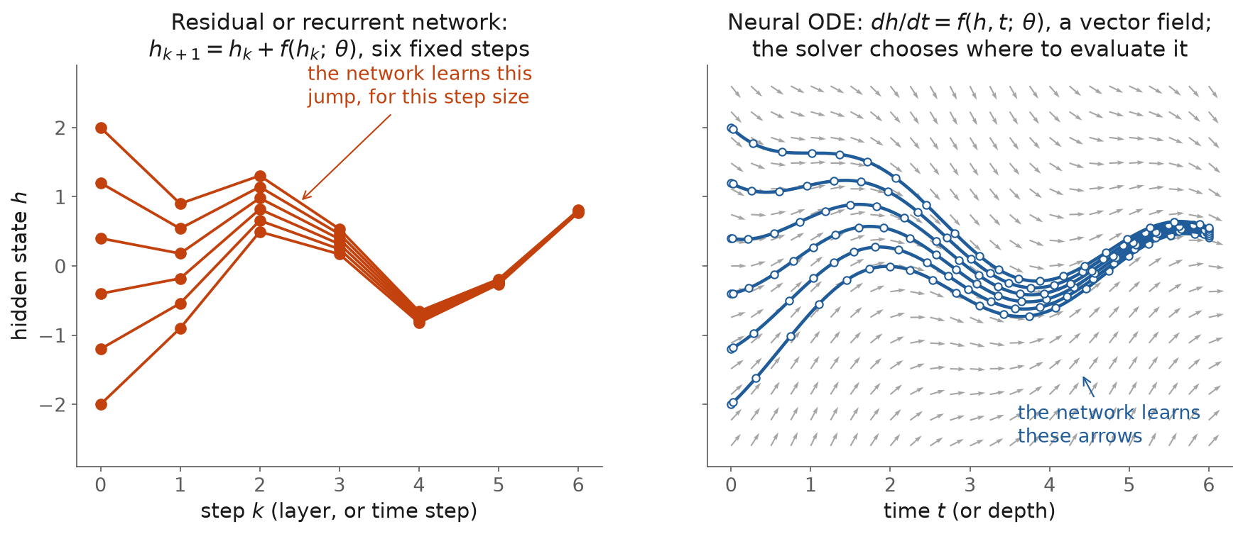
Fig. 86 A sequence of fixed steps (left) and a vector field with smooth trajectories (right), after Fig. 1 of Chen et al. (2018).

Takeaway: the vector field

A neural ODE learns the right-hand side \(f\): the vector field of the system. A recurrent network learns one time-discrete realization of it, tied to its step \(\Delta t\).

The same arrows hold for any starting state and any sampling times.

Neural ODEs and differentiable solvers

Definition: neural ODE

A neural ODE is a differential equation whose right-hand side is a neural network: \(\dfrac{dh}{dt} = f(h, t;\theta)\). An ODE solver computes the output.

Training a neural ODE:

1. Forward: start from \(h(t_0)\) and let the solver step to the measured times. Every step uses the same network \(f(\cdot;\theta)\).

2. Loss: compare \(h(t_i)\) with the data.

3. Backward: the gradient \(\partial L / \partial \theta\) has to come back through every solver step, because the loss depends on \(\theta\) through the whole simulation.

The gradient comes from a differentiable integrator:

• A solver written in JAX is a chain of differentiable operations.

• Reverse-mode automatic differentiation (Lecture 11) runs back through every solver step.

• Memory grows with the number of steps.

What you gain over a recurrent network:

• Any time points. The solver returns \(h\) at any \(t\), so irregular or missing samples are not a problem.

• The step size is the solver’s job, chosen to meet an error tolerance.

• The state can be physical: a temperature, a concentration.

Patrick Kidger’s work made neural ODEs practical tools.

• His Oxford thesis, On Neural Differential Equations (2021), calls neural networks and differential equations “two sides of the same coin”.

• With Morrill, Foster and Lyons he introduced neural controlled differential equations for irregularly sampled time series: “the Neural CDE is the continuous time analogue of an RNN” (2020).

• At Google X he built Diffrax, differentiable ODE solvers in JAX, and Equinox, neural networks in JAX.

A neural ODE for the bioreactor

The bioreactor balances are known; only \(\mu\) is learned:

\[\begin{split} \begin{aligned} \frac{dX}{dt} &= \mu X - \frac{F}{V}X, & \frac{dP}{dt} &= Y_{P/X}\,\mu X - \frac{F}{V}P, \\ \frac{dS}{dt} &= \frac{F}{V}(S_f - S) - \frac{\mu X}{Y_{X/S}}, & \frac{dV}{dt} &= F \end{aligned} \end{split}\]

\[ \mu = \mathrm{NN}(x;\theta), \qquad x = (X, P, S, V) \]

The network:

mu_scale = 0.3                                 # 1/h: sets the size of mu
x_typical = jnp.array([5.0, 1.0, 10.0, 3.0])   # typical X, P, S, V

class GrowthRate(eqx.Module):
    mlp: eqx.nn.MLP

    def __call__(self, x):
        out = self.mlp(x / x_typical)[0]       # any real number
        return mu_scale * jax.nn.softplus(out) # mu >= 0, of order mu_scale

• eqx.Module is Equinox’s network class; eqx.nn.MLP is a multilayer perceptron.

• x / x_typical divides each state by a typical value, so the network sees numbers near 1.

• softplus is always positive, so \(\mu \ge 0\). At the start of training softplus is about 0.7, so \(\mu\) starts near \(0.3 \times 0.7 \approx 0.2\) 1/h, a sensible growth rate. That is what mu_scale is for.

• Nothing keeps \(S \ge 0\).

Universal differential equation (UDE)

A mechanistic model with one term a network is also called a universal differential equation: “differential equations which are defined in full or part by a universal approximator” (Rackauckas et al., 2020). Neural ODE, UDE and hybrid model are used interchangeably for this.

The right-hand side of the ODE:

def balances(t, x, args):
    mu_net, Sf = args
    X, P, S, V = x
    mu = mu_net(x)                               # the learned term
    dX = mu * X - F / V * X
    dP = Ypx * mu * X - F / V * P
    dS = F / V * (Sf - S) - mu * X / Yxs
    dV = F
    return jnp.array([dX, dP, dS, dV])

The solve, with Diffrax:

def simulate(mu_net, x0, ts):
    sol = diffrax.diffeqsolve(
        diffrax.ODETerm(balances),
        diffrax.Tsit5(),
        t0=0.0,
        t1=ts[-1],
        dt0=0.1,
        y0=x0,
        args=(mu_net, x0[2]),
        saveat=diffrax.SaveAt(ts=ts),
        stepsize_controller=diffrax.PIDController(
            rtol=1e-6,
            atol=1e-8,
        ),
    )
    return sol.ys

• ODETerm(balances): the right-hand side.

• Tsit5(): Tsitouras’ fifth-order Runge-Kutta method.

• t0, t1, dt0, y0: from time 0 to the last sample, first step 0.1 h, from the initial state. args passes the network and the feed concentration to balances.

• SaveAt(ts=ts): return the states at the sample times. PIDController: adapt the step to keep the error below the tolerances.

• Every operation is JAX, so jax.grad of anything computed from sol.ys goes back through the solver.

Training is the sequential approach: every step simulates the three batches, compares with the data, and updates the weights.

def loss(mu_net):
    pred = jax.vmap(simulate, in_axes=(None, 0, None))(mu_net, x0s, ts)
    return jnp.mean(((pred - ys) / y_scale) ** 2)

mu_net = GrowthRate(eqx.nn.MLP(
    in_size=4,
    out_size=1,
    width_size=16,
    depth=2,
    activation=jnp.tanh,
    key=jax.random.PRNGKey(0),
))
opt = optax.adam(optax.cosine_decay_schedule(1e-2, steps, alpha=0.05))
state = opt.init(eqx.filter(mu_net, eqx.is_array))

@eqx.filter_jit
def step(mu_net, state):
    value, grads = eqx.filter_value_and_grad(loss)(mu_net)
    updates, state = opt.update(grads, state, mu_net)
    return eqx.apply_updates(mu_net, updates), state, value

for _ in range(10_000):
    mu_net, state, value = step(mu_net, state)

• The loss compares the three simulated batches with their 31 samples, each state divided by its spread in the data.

• Adam’s learning rate decays from 0.01 along a cosine. 10,000 steps take about 35 s.

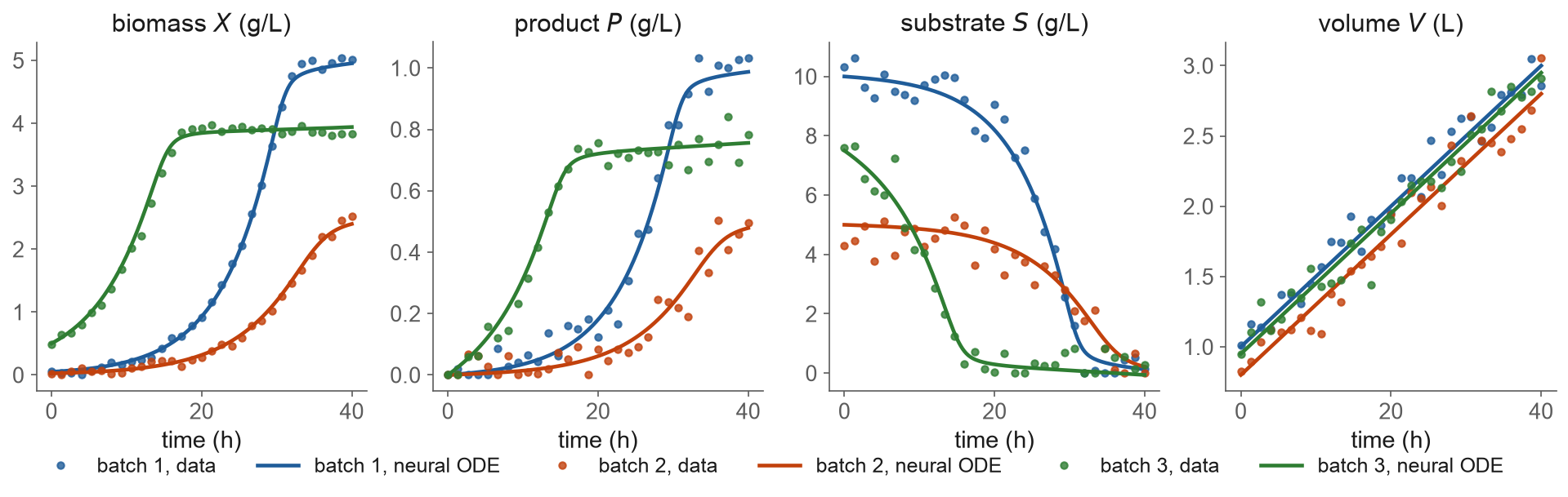
Fig. 87 Three training batches, 31 noisy samples of each state (dots), and the trained neural ODE (lines).

• Against the true model, the fit is off by 0.047 g/L in \(X\) and 0.094 g/L in \(S\): within the measurement noise (0.05 and 0.5 g/L).

• The measurements follow the SiNDAE fed-batch example: the true model, where \(\mu\) follows the Monod law \(\mu = \mu_\text{max} S/(K_S + S)\), plus noise. A reading below zero is recorded as zero. The network never sees that law.

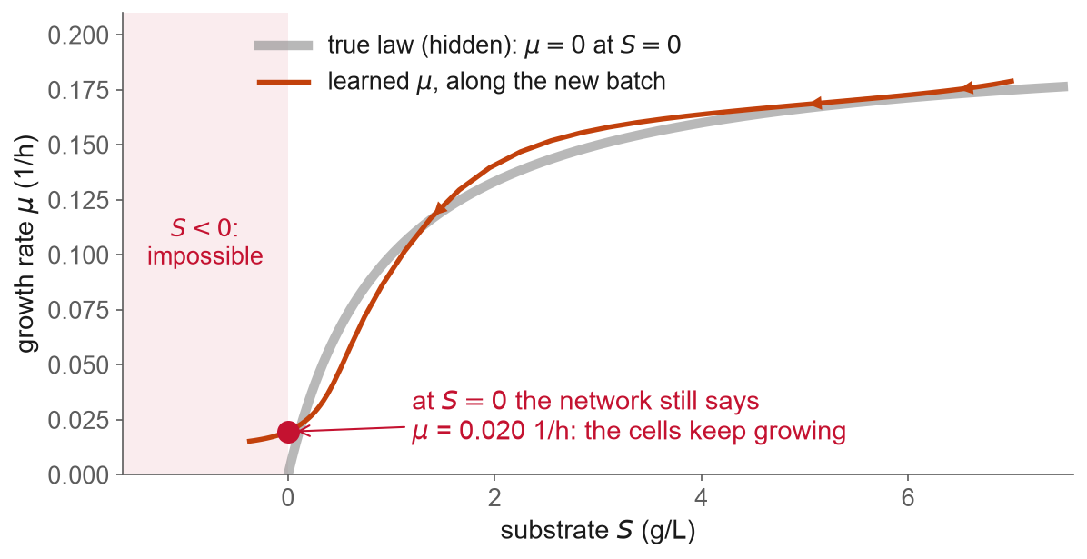
Fig. 88 The learned growth rate along the new batch.

• Takeaway: the network learned \(\mu\) well where the data were. It was never told that cells cannot grow without substrate, so at \(S = 0\) (38 h on the new batch) it still gives \(\mu = 0.020\) 1/h, and the balances drive \(S\) below zero.

• The balances hold the whole time. Nothing in the model says that \(S\) cannot be negative.

Physics-enforced machine learning

Gen 2 promised guaranteed constraints. A PINN only informs the training with the physics. For some physics that is not enough.

From a penalty to a constraint

\[ \underbrace{\min_\theta\; L_\text{data} + \lambda\,\lVert r \rVert^2}_{\text{informed: } r \text{ small}} \qquad\longrightarrow\qquad \underbrace{\min_\theta\; L_\text{data} \quad \text{s.t.}\quad r = 0,\;\; g \le 0}_{\text{enforced: } r = 0 \text{ to solver tolerance}} \]

A hard constraint holds at the solution to solver tolerance. Why enforce:

• Conservation. Mass and energy balances must close.

• Safety. A reactor temperature or a pressure must stay below its limit at every instant.

• Physical bounds. Concentrations cannot be negative, the \(S < 0\) above.

• Quality and regulation. A product specification must be met, not approached.

• No \(\lambda\) to tune, and the guarantee holds outside the training data too.

Path constraints

Definition: path constraint

A path constraint is an inequality on the states that must hold at every instant: \(g\big(x(t)\big) \le 0\) for all \(t\).

• “Problems of dynamic optimisation with inequality path constraints are common in industrial plants. These constraints describe conditions of the process when it operates with extreme values of the variables, based on safety and/or economics restraints” (Souza et al., 2006).

• A batch reactor: limits on cooling duty and “an adiabatic temperature rise constraint that enforces safe operation even if cooling is lost” (Biegler, 2017).

• A plate reactor start-up: “a temperature path constraint, which is straight forward to enforce using a simultaneous method” (Haugwitz et al., 2007).

• Our bioreactor: \(S(t) \ge 0\) for all \(t\).

Differential-algebraic equations

Definition: differential-algebraic equation (DAE)

A DAE is a set of differential equations plus algebraic equations that hold at every instant.

\[ \frac{dx}{dt} = f(x, y), \qquad 0 = g(x, y) \]

• \(x\) are the differential states: they have a derivative in the model (levels, concentrations, temperatures).

• \(y\) are the algebraic variables: no derivative, set at every instant by \(g = 0\) (flows, pressures, rates).

• An ODE is the special case with no \(g\).

• Process models are full of algebraic equations: vapor-liquid equilibrium in a flash drum, flows that balance at a node, flow through a valve.

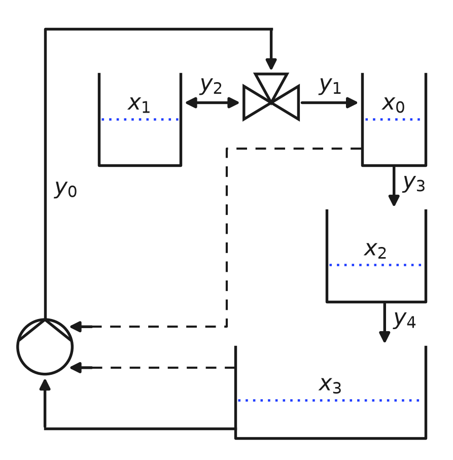
Fig. 89 A tank manifold. Levels \(x_0\) to \(x_3\); flows \(y_0\) to \(y_4\). Redrawn from Lueg et al. (2026), Fig. 1 (CC BY 4.0).

Part of its model:

\[ \frac{dx_0}{dt} = \frac{y_1 - y_3}{\phi_0}, \qquad \frac{dx_1}{dt} = \frac{y_2}{\phi_1}, \qquad y_0 = y_1 + y_2, \qquad \underbrace{x_0 = x_1}_{\text{equal levels}} \]

• \(\phi_i\) is the cross-sectional area of tank \(i\).

• No equation gives \(y_2\) directly. It is whatever keeps \(x_0 = x_1\) at every instant.

• An algebraic equation is a constraint that holds all the time: what we want to enforce.

Neural DAEs: the spring-mass with the physics enforced

Back to the PINN’s spring-mass. Suppose the damping is the unknown. Make it the network output \(z\), and move the equation from the loss into the constraints:

\[\begin{split} \begin{aligned} \min_\theta\quad & \sum_i \big(x(t_i) - \hat x_i\big)^2 \\ \text{s.t.}\quad & m\,x'' + z\,x' + k\,x = 0 \\ & z = \mathrm{NN}(x, x';\theta) \\ & h(x) = 0, \quad g(x) \le 0 \end{aligned} \end{split}\]

The physics is now enforced, rather than informed: the equation is a constraint of the optimization problem.

Definition: neural DAE

A neural DAE is a DAE in which some unknown terms are neural networks, trained with the simultaneous approach of the next section.

Lueg, Alves, Schicksnus, Kitchin, Laird and Biegler train neural DAEs this way (Computational Optimization and Applications, 2026, open access; arXiv).

Training a dynamic model: sequential or simultaneous

Fitting a dynamic model to data is an optimization problem with the model as a constraint:

\[ \min_{\theta} \;\sum_i \big(x(t_i) - \hat x_i\big)^2 \quad \text{subject to} \quad \frac{dx}{dt} = f(x;\theta), \;\; x(0) = x_0 \]

• \(\hat x_i\) are the measurements; \(\theta\) are the unknown parameters (or network weights).

• This is a dynamic optimization problem. There are two classic ways to solve it (Biegler, 2007).

• The example: the spring-mass, lightly damped (true \(\mu = 1\) N·s/m, \(k = 400\) N/m), 51 noisy measurements over 2 s (noise standard deviation 0.03 m). Estimate \(\mu\) and \(k\) from a poor starting guess, \(\mu = 2\) and \(k = 150\).

Sequential: simulate, then optimize

Definition: sequential approach (single shooting)

The sequential approach guesses \(\theta\), simulates the model with an ODE solver, computes the loss and its gradient, updates \(\theta\), and repeats.

\[\begin{split} \begin{aligned} &\text{1. Guess:} && \theta_0 \\ &\text{2. Simulate:} && x(t;\theta) = \mathrm{ODESolve}(f, x_0, \theta) \\ &\text{3. Loss and gradient:} && L(\theta) = \sum_i \big(x(t_i;\theta) - \hat x_i\big)^2, \quad \nabla_\theta L \\ &\text{4. Update, and back to 2:} && \theta \leftarrow \theta - \eta\,\nabla_\theta L \end{aligned} \end{split}\]

Fig. 90 One pass of the sequential loop: guess, simulate, compare, update. The last panel is the loss after each update.

• Every iterate is a full simulation: the model holds at every step.

• Training the neural ODE above with Diffrax and Adam was sequential.

• Biegler: “sequential approaches are known to fail on unstable dynamic systems” (FOCAPO/CPC 2017).

• The loss over \((\mu, k)\) has one narrow valley along \(k\): an oscillation slightly out of phase fits the data badly everywhere.

Simultaneous: discretize, then optimize

Definition: simultaneous approach (collocation)

The simultaneous approach turns the state at every time point into an unknown, writes the differential equation as algebraic equations between those points, and solves one large optimization problem for the states and \(\theta\) together.

From one simulated curve to one optimization problem:

1. Cut the time horizon into finite elements.

2. Every state at every point of every element becomes an unknown, started on the data.

3. At the start the model equations do not hold: one residual per point.

4. One solver moves all the points and \(\theta\) together, until every equation holds.

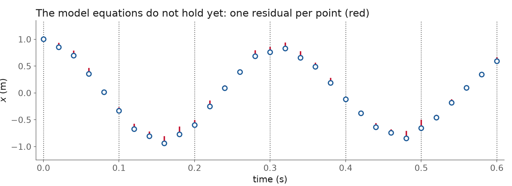
Fig. 91 The starting point of the simultaneous approach: states on the data, model equations broken.

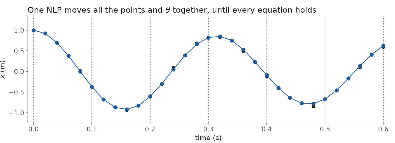
Fig. 92 The solved problem: the points form a trajectory that obeys the model.

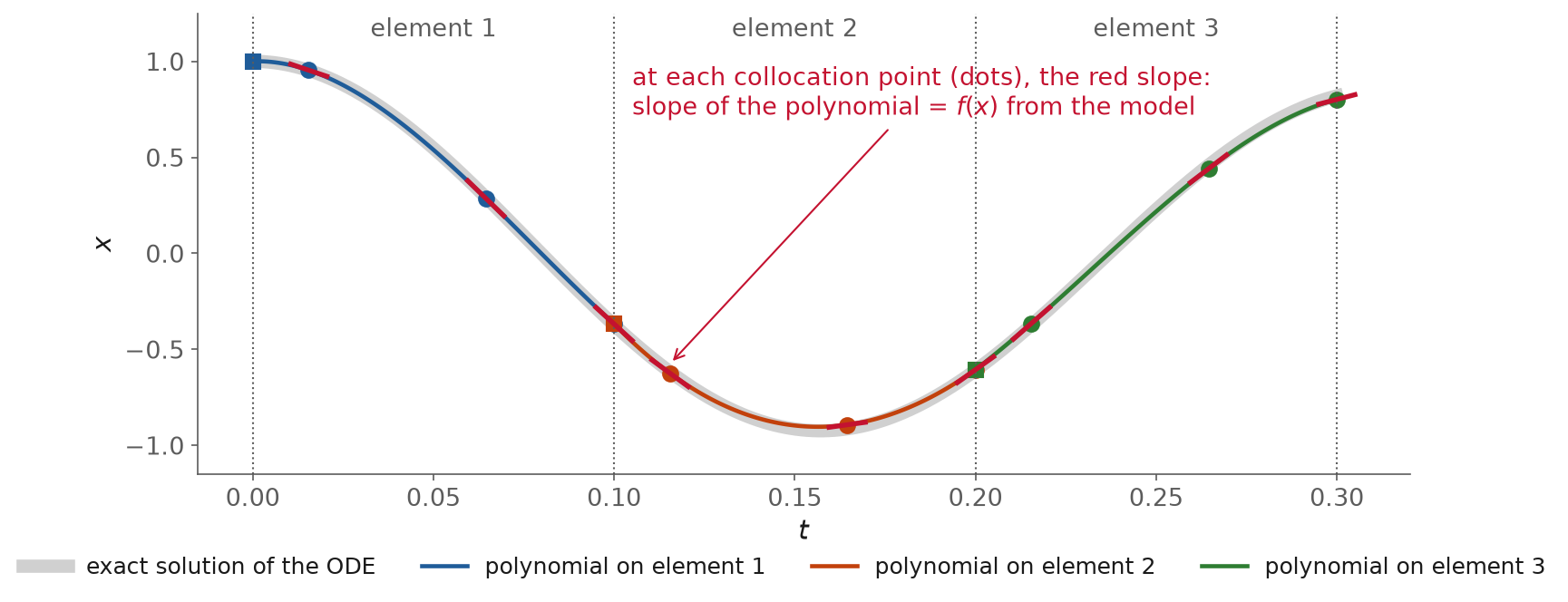
Fig. 93 Collocation on the spring-mass, solved: on each element a cubic whose slope equals the model’s slope at three collocation points. It stays close to the exact solution.

On each finite element \(j\) the state is a polynomial through \(K + 1\) points. Its values \(x_{jk}\) at those points are unknowns of the NLP. At each collocation point \(t_{jk}\) the polynomial’s slope must equal the slope the model gives:

\[ \underbrace{\frac{dx_\text{poly}}{dt}(t_{jk})}_{\text{slope of the polynomial}} \;=\; \underbrace{f\big(x_{jk};\theta\big)}_{\text{slope from the model}}, \qquad k = 1, \dots, K \]

• The polynomial’s slope at a point is a fixed weighted sum of its point values \(x_{j0}, \dots, x_{jK}\), so each equation is algebraic in the unknowns.

• This is orthogonal collocation on finite elements. The equations in full: Biegler (2007), and his lecture slides on collocation (open).

This is the constrained optimization problem of Lecture 9, \(\min_z f(z)\) subject to \(h(z) = 0\) and \(g(z) \le 0\), with \(z\) every state value and \(\theta\):

\[\begin{split} \begin{aligned} \min_{\theta,\;x_{jk}}\quad & \sum_i \big(x(t_i) - \hat x_i\big)^2 && \text{fit the data} \\ \text{s.t.}\quad & \frac{dx_\text{poly}}{dt}(t_{jk}) = f(x_{jk};\theta) && \text{polynomial slope = model slope} \\ & x_{j,K} = x_{j+1,0} && \text{elements join} \\ & x_{1,0} = x_0 && \text{initial condition} \\ & g(x_{jk}) \le 0 && \text{path constraints} \end{aligned} \end{split}\]

• The result is one nonlinear program (NLP). Pyomo.DAE writes the discretized equations from the continuous model, and IPOPT, an interior-point NLP solver, solves it.

• The model equations are satisfied only when the solver converges. Biegler: “the dynamic system is solved only once, at the optimal point.”

The same problem, both ways

• Sequential: a Runge-Kutta simulation inside BFGS, a gradient-based optimizer.

• Simultaneous: trapezoidal collocation on 200 steps, solved by the POUNCE interior-point solver. 404 unknowns: two states at 201 points, plus \(\mu\) and \(k\).

Scrub through the iterations of each:

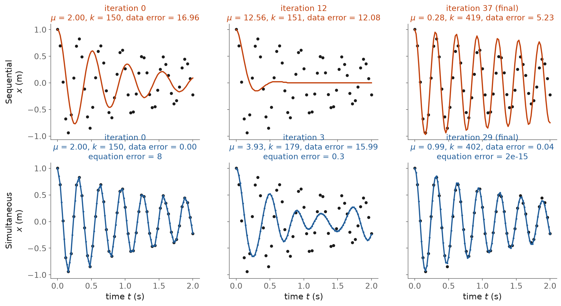
Fig. 94 Selected iterations. Data error: the sum of squared errors (SSE) over the 51 measurements. Equation error: how far the model equations are from holding, the largest violation of the collocation equations.

From \(\mu = 2\), \(k = 150\)	Sequential	Simultaneous
Iterations	37 (BFGS)	29 (interior point)
Final \(\mu\), \(k\)	0.29, 419	0.99, 402
Sum of squared errors	5.23	0.036
Model equations satisfied	at every iterate	from 7.7 at the start to \(2.5 \times 10^{-15}\) at the end

• The sequential run gets stuck in a local minimum. Its trajectory oscillates at nearly the right frequency but keeps too much amplitude.

• The simultaneous run starts with the states on the data (so it fits, but breaks the ODE), then pulls the two together. It ends at the true parameters, within noise (with the true values the sum of squared errors is 0.038).

• From a better guess (\(k\) = 250, 350 or 450) both methods find \(\mu \approx 0.98\) and \(k \approx 400\).

Trade-offs

	Sequential	Simultaneous
Model holds at every iterate	yes	only at convergence
Unknowns	the parameters	parameters + every state at every point
Solver	ODE solver + gradient method (Adam, BFGS)	NLP solver (IPOPT, POUNCE)
Oscillating or unstable dynamics	can stall in a local minimum	states pinned to the data
Path constraints (\(S \ge 0\))	penalties, checked afterwards	rows of the NLP, enforced
DAEs	must be rewritten as ODEs first	written at the collocation points
Time steps	adaptive, error-controlled	a fixed grid, chosen beforehand
Big data, big networks	mini-batches on GPUs	the NLP grows with the data

Between the two sits multiple shooting: simulate short segments, and make their ends meet as constraints.

Training neural DAEs

The training problem

For trajectories (batches, experiments) \(s\), the problem is (their Eq. 4):

\[\begin{split} \begin{aligned} \min_{\theta,\,x,\,y,\,z}\quad & \underbrace{\sum_{s} \sum_{i} \big\|x^{(s)}(t_i) - \hat x_i^{(s)}\big\|^2}_{\text{every trajectory}} \;+\; \underbrace{\alpha_r\, \tfrac{1}{2}\|\theta\|^2}_{\text{regularization}} \\ \text{s.t.}\quad & \frac{dx^{(s)}}{dt} = f\big(x^{(s)}, y^{(s)}, z^{(s)}\big) && \text{differential equations} \\ & 0 = h\big(x^{(s)}, y^{(s)}, z^{(s)}\big) && \text{algebraic equations} \\ & 0 \ge g\big(x^{(s)}, y^{(s)}, z^{(s)}\big) && \text{inequalities } (S \ge 0) \\ & z^{(s)} = f_\text{NN}\big(x^{(s)};\theta\big) && \text{the network: the unknown terms} \\ & x^{(s)}(t_0) = x_0^{(s)} && \text{initial conditions} \end{aligned} \end{split}\]

• Every line holds at every collocation point of every trajectory, so the physics is exact at the solution.

• One \(\theta\) is shared by all trajectories, so one network fits every batch at once, and is reusable for new starting charges and feed profiles.

• Smooth activations (tanh, softplus, not ReLU): the interior-point solver uses second derivatives of the network.

Making it solvable

The full NLP is large and nonconvex. Started cold, it can fail or be slow. The paper solves it in three steps:

1. Smoother. Solve the problem without the network: the unknown terms \(z\) are free functions of time, kept smooth by a penalty. This gives consistent trajectories close to the data.

2. Pretrain. Fit the network to the smoother’s \((x, z)\) pairs with Adam. Now the weights start near a good answer.

3. Full NLP. Solve the network, the states and the balances together, from steps 1 and 2.

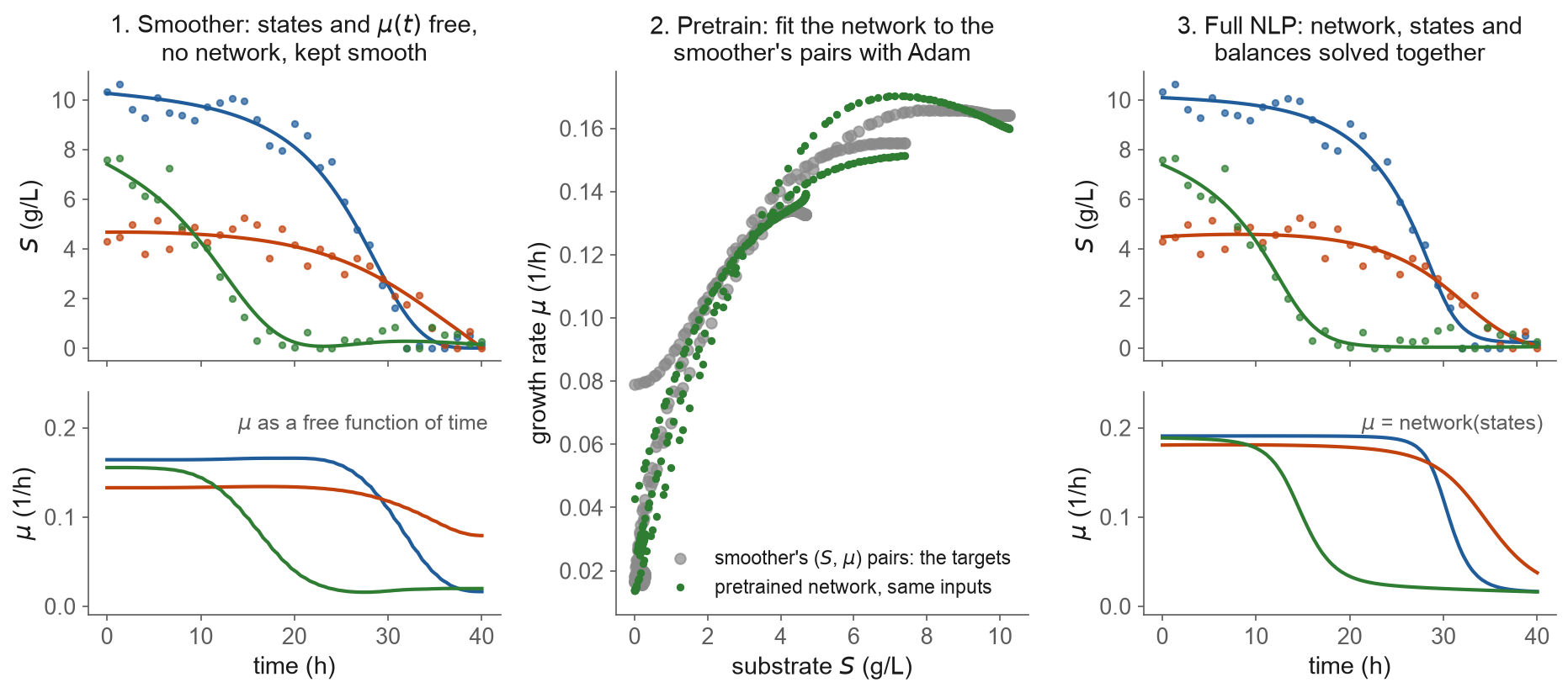
Fig. 95 The three stages on the bioreactor’s three training batches.

Inference on a new batch

Definition: inference

Inference is using the trained model to predict a case it has never seen, with the network weights fixed.

Both models learned \(\mu\) from the same three batches. The new batch starts with 0.2 g/L of cells, 7 g/L of substrate and 0.9 L, and runs for 60 h, 20 h past the training batches.

• Neural ODE: integrate the learned model, the sequential way.

• Neural DAE: solve the same balances as an NLP with \(S \ge 0\), the simultaneous way.

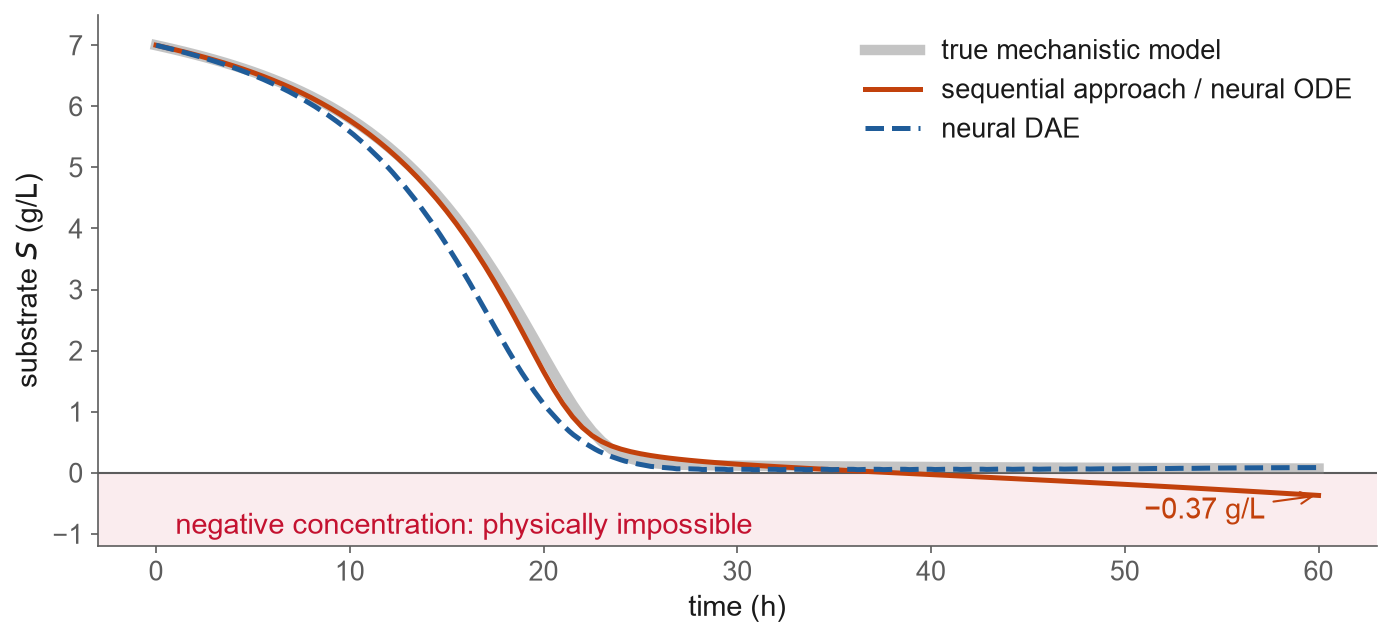
Fig. 96 The new batch: the true mechanistic model, the neural ODE and the neural DAE.

New batch, 60 h	True mechanistic model	Sequential approach / neural ODE	Neural DAE
Lowest substrate \(S\)	0.07 g/L	−0.37 g/L	0.05 g/L
Hours with \(S < 0\)	0	22	0
Substrate error (RMSE)		0.19 g/L	0.30 g/L
Biomass \(X\) at 60 h	3.51 g/L	3.73 g/L	3.50 g/L

• In prediction, SiNDAE lets the solver move the growth rate away from the network’s value only where a constraint would otherwise break, at a price set by slack_coef.

• Feasible is not the same as accurate. The constraint keeps the prediction physical; it does not make the learned growth rate correct. Here the neural DAE’s substrate error is larger than the neural ODE’s.

SiNDAE

SiNDAE (Simultaneous Neural Differential-Algebraic Systems of Equations) is a Python package that learns unknown terms in dynamical systems from noisy time series while fully satisfying the constraints.

• Mechanistic equations are kept as hard constraints, so the model stays physically consistent, also for conditions never seen in training.

• The network sits inside the model, trained by solving one constrained NLP with an interior-point method.

• Install: pip install sindae. No licensed solver is needed.

• Code and docs: github.com/Alves-research-group/SiNDAE, documentation.

What it is built on, and what each part does:

Role	Tool	What it does here
Physics modeling	Pyomo	writes the model’s equations and constraints
	Pyomo.DAE	derivatives in time, and their discretization
Machine learning	JAX	the network and its derivatives
	ONNX	a file format to export the trained network
	OMLT	puts trained networks into Pyomo models
Constrained optimization	IPOPT	interior-point solver for the NLP
	POUNCE	interior-point solver, no license needed

The code follows the SiNDAE example Importing Measured Data, Fed-Batch Bioreactor, with the product balance diluted by \(F/V\).

The class. A SiNDAE problem is a subclass of ProblemDefinition:

class FedBatchBioreactorProblem(ProblemDefinition):
    def __init__(
        self,
        params,
        ics,
        input_dim,
        z_dim,
        t_span,
        nfe,
        ncp,
        obs_times=None,
        obs_values=None,
        obs_dim=None,
    ):
        super().__init__(ics, input_dim, z_dim, t_span, nfe, ncp,
                         obs_times, obs_values, obs_dim)
        self.params = params

• The arguments: the initial charge of each batch (ics), 4 states and 1 learned term, the time span, the finite elements and collocation points, and the measurements.

• ProblemDefinition stores them; the class adds our parameters, the feed rate and the yields.

The variables. build_trajectory, a method of the same class, writes the model for one batch in Pyomo:

    def build_trajectory(self, block, traj_idx):
        p = self.params
        t0 = self.t_span[0]
        x0 = self.ics[traj_idx]
        Sf = float(x0[2])                # feed concentration = initial substrate
        Feed, Ypx, Yxs = p["Feed"], p["Ypx"], p["Yxs"]

        block.t = dae.ContinuousSet(bounds=self.t_span)
        block.x = pyo.Var(
            block.t,
            range(self.input_dim),
            domain=pyo.NonNegativeReals,
            initialize=1.0,
        )
        block.z = pyo.Var(block.t, range(self.z_dim), initialize=0.1)
        block.dxdt = dae.DerivativeVar(block.x, wrt=block.t)

• It is called once per batch, with that batch’s initial charge.

• ContinuousSet: time, continuous; Pyomo.DAE discretizes it later.

• NonNegativeReals declares every state non-negative: here is \(S \ge 0\).

• z is \(\mu\): a free variable the network will set. dxdt are the derivatives of the states.

The balances, the initial charge, and the network’s inputs and output:

        @block.Constraint(block.t, range(self.input_dim))
        def diffeq(b, t, s):
            mu = b.z[t, 0]               # growth rate, learned by the network
            X, P, S, V = b.x[t, 0], b.x[t, 1], b.x[t, 2], b.x[t, 3]
            if s == 0:
                return b.dxdt[t, 0] == mu * X - Feed * (X / V)
            elif s == 1:
                return b.dxdt[t, 1] == Ypx * mu * X - Feed * (P / V)
            elif s == 2:
                return b.dxdt[t, 2] == Feed * (Sf - S) / V - mu * (X / Yxs)
            else:
                return b.dxdt[t, 3] == Feed

        for j in range(self.input_dim):
            block.x[t0, j].fix(float(x0[j]))

    def get_input_vars(self, block, t):
        return [block.x[t, j] for j in range(self.input_dim)]

    def get_output_vars(self, block, t):
        return [block.z[t, 0]]

• A constraint for every time \(t\) and every state \(s\): these are rows of the NLP.

• One balance per branch. There is no formula for \(\mu\).

• get_input_vars and get_output_vars connect the network: the states in, \(z = \mu\) out.

The network and the three training stages:

mlp = SimpleMLP(
    in_size=INPUT_DIM,
    out_size=Z_DIM,
    widths=[20, 20],
    activations=[jax.nn.softplus] * 2,
    key=jax.random.PRNGKey(SEED),
)
smoother_config = SmootherConfig(smooth_coef=10.0)
pretrain_config = PretrainConfig(
    epochs=200,
    batch_size=32,
    reg_coef=1e-3,
)
simul_config = SimultaneousConfig(
    use_gbm=True,
    reg_coef=1e-3,
)
solver_options = SolverConfig(
    tol=1e-6,
    max_iter=1000,
)

• SimpleMLP: 4 states in, \(\mu\) out, two hidden layers of 20 softplus units. Softplus is smooth, as the interior-point solver needs.

• SmootherConfig, PretrainConfig and SimultaneousConfig are the three stages above.

• use_gbm=True hands the network to the solver as an external function evaluated in JAX, so SiNDAE approximates the second derivatives of that solve with L-BFGS. The smoother has no network and uses exact second derivatives.

Training. Attach the measurements of the three batches, then fit:

problem = FedBatchBioreactorProblem(
    params=FB_PARAMS,
    ics=BATCH_ICS,
    input_dim=INPUT_DIM,
    z_dim=Z_DIM,
    t_span=T_SPAN,
    nfe=NFE_TRAIN,
    ncp=NCP_TRAIN,
    obs_dim=OBS_DIM,
    obs_times=obs_times,
    obs_values=obs_values,
)

model = HybridDAE(
    method="simultaneous",
    nlp_solver="pounce",
    net=mlp,
    smoother=smoother_config,
    pretrain=pretrain_config,
    train=simul_config,
    solver_options=solver_options,
    unfix_io=True,
)
model.fit(problem)

• Training uses 40 finite elements of 3 collocation points over 40 h; this grid need not match the 31 samples.

• fit runs the smoother, the pretraining and the full NLP, solved by POUNCE. About 30 s.

Prediction on the new batch:

new_problem = FedBatchBioreactorProblem(
    params=FB_PARAMS,
    ics=np.array([[0.20, 0.0, 7.0, 0.90]]),
    input_dim=INPUT_DIM,
    z_dim=Z_DIM,
    t_span=(0.0, 60.0),
    nfe=45,
    ncp=3,
    obs_dim=OBS_DIM,
)
prediction = model.predict(
    new_problem,
    slack_coef=1e-5,
)

• The same class, a new initial charge, 60 h and no measurements.

• predict solves the DAE with the network fixed and \(S \ge 0\) held. slack_coef is the price on moving \(\mu\) away from the network’s value where a constraint would otherwise break.

Case study: monoclonal antibody production

Monoclonal antibodies (mAbs) are medicines for cancers and for autoimmune and infectious diseases. Most are made by CHO cells in fed-batch reactors.

• Glycosylation is the attachment of sugar chains (glycans) to the antibody inside the cell, finished in the Golgi apparatus.

• The glycans are a critical quality attribute (CQA): a property that “must be within an appropriate limit, range or distribution to ensure the desired product quality, safety and efficacy”. For mAbs, “the terminal sugars of Fc glycans have been shown to be critical for safety or efficacy” (Reusch and Tejada, 2015).

• Glycans also change how the drug behaves in the body and immune reactions to it.

A hybrid glycosylation model from the Alves group (a proof of concept):

• 9 states: viable cells, glucose, glutamine, lactate, ammonia, the antibody, and three glycoforms G0F, G1F and G2F.

• Mechanistic: six culture balances, and three glycan equations.

• Algebraic: the nucleotide sugar donors (NSDs), the sugar building blocks, are at quasi-steady state, set by glucose at every instant. That makes the model a DAE.

• Learned: the growth rate, \(\mu = f_\text{NN}(x;\theta)\), a network with 9 inputs, two hidden layers of 16 tanh units, and 1 output.

• Why \(\mu\): it is never measured, and its usual law (Monod kinetics, inhibited by lactate and ammonia) is an assumption.

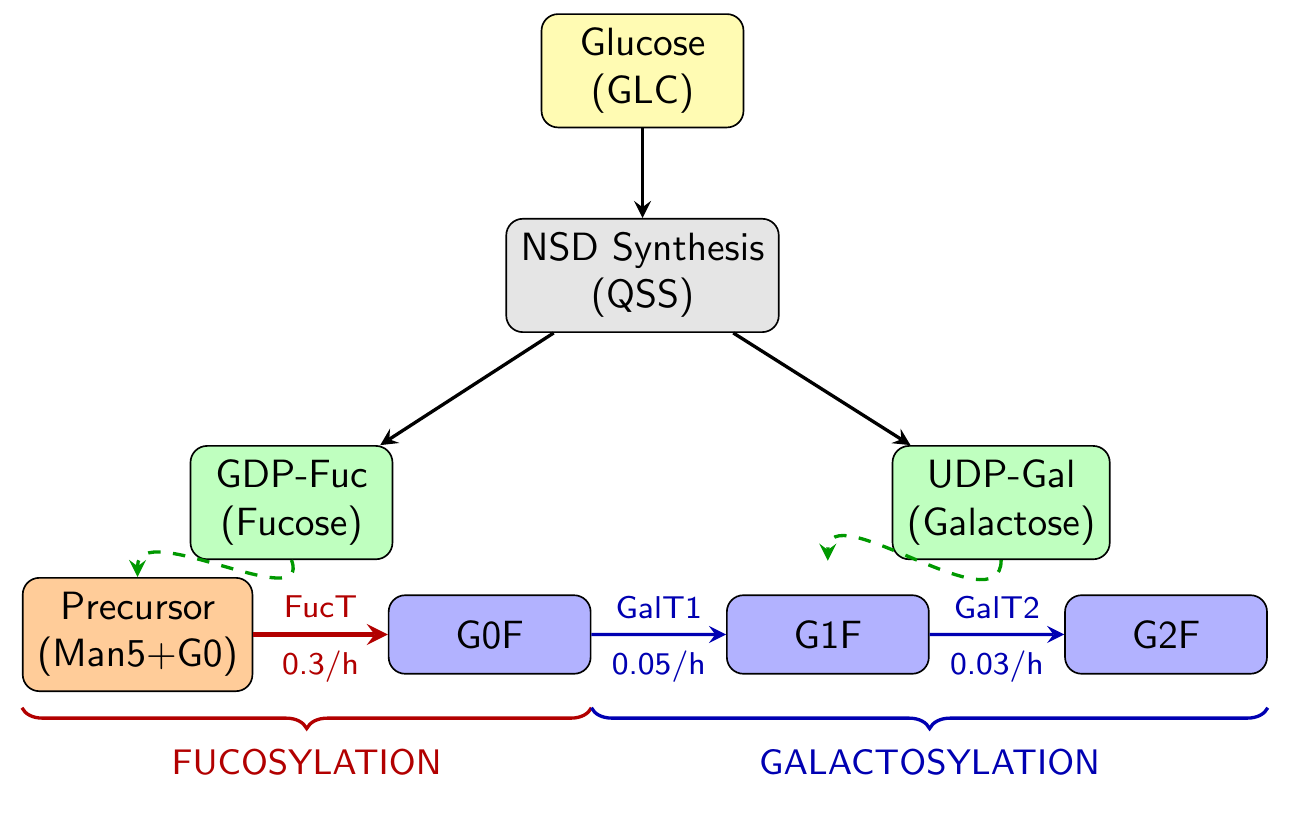
Fig. 97 The glycosylation steps in the model: fucosylation, then two galactosylations.

The equations, by scale. The learned term is \(\mu\), at the process scale:

\[\begin{split} \begin{aligned} \frac{dX_v}{dt} &= (\mu - \mu_d)\,X_v \\ \frac{dGLC}{dt} &= -\Big(\frac{\mu - \mu_d}{Y_{X_v/glc}} + m_{glc}\frac{GLC}{K_{glc} + GLC}\Big)X_v \\ &\;\;\vdots \\ \mu &= f_\text{NN}(x;\theta) \end{aligned} \end{split}\]

At the cell scale, the sugar donors are algebraic (quasi-steady state):

\[ \text{UDP-Gal} = \frac{V_{max,Gal}\,GLC}{K_{M,Gal} + GLC}, \qquad \text{GDP-Fuc} = \frac{V_{max,Fuc}\,GLC}{K_{M,Fuc} + GLC} \]

At the Golgi scale, the glycans, with \(\phi_{Gal} = \text{UDP-Gal}/(K_{UDP\text{-}Gal} + \text{UDP-Gal})\) and \(\phi_{Fuc} = \text{GDP-Fuc}/(K_{GDP\text{-}Fuc} + \text{GDP-Fuc})\):

\[\begin{split} \begin{aligned} \frac{dG0F}{dt} &= k_{FucT}\,\text{Pre}\;\phi_{Fuc} - k_{GalT1}\,G0F\;\phi_{Gal} \\ \frac{dG1F}{dt} &= k_{GalT1}\,G0F\;\phi_{Gal} - k_{GalT2}\,G1F\;\phi_{Gal} \\ \frac{dG2F}{dt} &= k_{GalT2}\,G1F\;\phi_{Gal} \\ \text{Pre} &= 1 - G0F - G1F - G2F \end{aligned} \end{split}\]

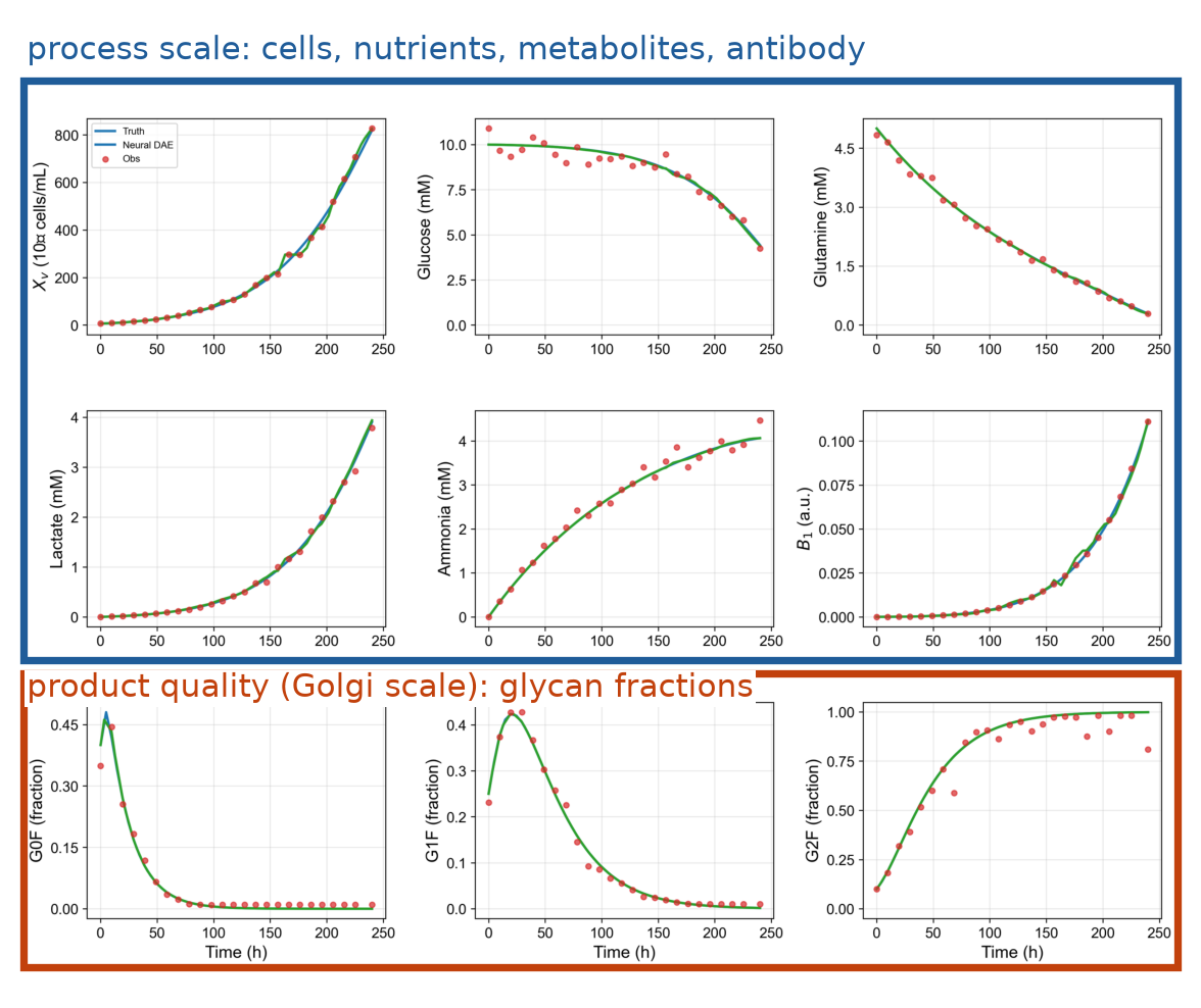
Fig. 98 One model fitted to data at two scales: process measurements (blue box) and glycan fractions (orange box). True model (blue), neural DAE (green), noisy data (red).

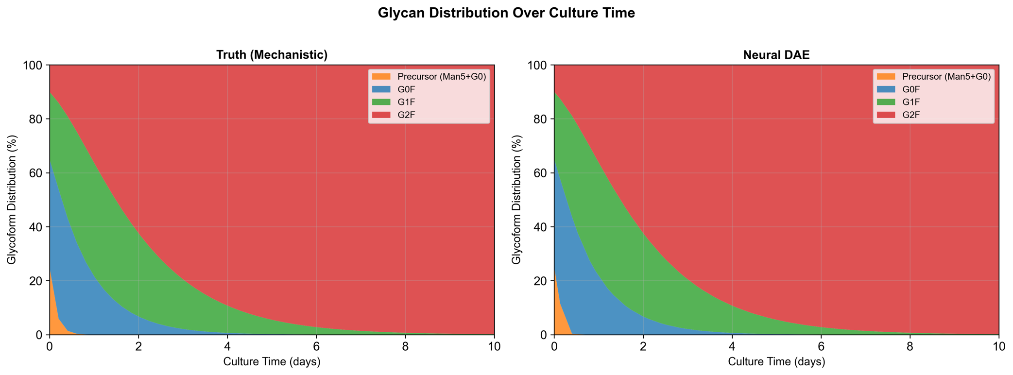
Fig. 99 Glycan composition over the culture: true model (left) and neural DAE (right).

• The data are synthetic: the mechanistic model plus noise, half of the samples kept, three runs of 10 days.

• Limits: 3 of more than 33 glycoforms; quasi-steady sugar donors; the learned \(\mu(t)\) oscillates even though the states fit.

Constraints inside the network: projection layers

A neural DAE enforces constraints in the solver. Another option is to build them into the network, so that every output satisfies them.

Projection layers

Definition: projection layer

A projection layer is a last layer that moves the network’s raw output \(\tilde y\) to the closest point that satisfies the constraints.

The example: a heat exchanger that must not create energy. Hot water at 90 °C heats cold water at 20 °C and 1 kg/s in a counterflow exchanger.

• Input: the hot-water flow \(\dot m_h\), from 0.2 to 2 kg/s.

• Outputs: the two outlet temperatures, \(y = (T_{h,out},\ T_{c,out})\).

• First law: the heat the hot water gives up is the heat the cold water takes.

\[ \underbrace{\dot m_h c_p\,(T_{h,in} - T_{h,out})}_{Q_h:\ \text{heat given up}} \;=\; \underbrace{\dot m_c c_p\,(T_{c,out} - T_{c,in})}_{Q_c:\ \text{heat taken}} \]

• A network that predicts the two temperatures can break it: \(Q_c > Q_h\) is energy from nothing.

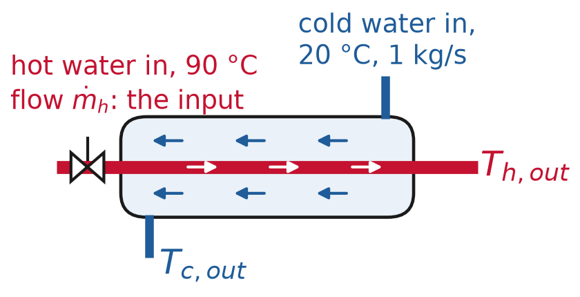
Fig. 100 The counterflow heat exchanger.

The balance is linear in the outputs:

\[ \underbrace{\dot m_h\,T_{h,out} + \dot m_c\,T_{c,out}}_{a^\top y} \;=\; \underbrace{\dot m_h\,T_{h,in} + \dot m_c\,T_{c,in}}_{b}, \qquad a = (\dot m_h,\ \dot m_c) \]

\[ u \;\longrightarrow\; \underbrace{\mathrm{NN}(u;\theta)}_{\text{network}} \;\longrightarrow\; \tilde y \;\longrightarrow\; \underbrace{P(\tilde y)}_{\text{projection}} \;\longrightarrow\; y \;\longrightarrow\; \text{loss} \]

The closest point to the raw output \(\tilde y\) that obeys the balance:

\[ v = a^\top \tilde y - b, \qquad y = \tilde y - \frac{a\,v}{a^\top a} \]

• \(v\) is how much the raw output breaks the balance: \(c_p v = Q_c - Q_h\).

• The correction is linear in \(\tilde y\), with no trainable weights. \(a\) and \(b\) change with the input flow; the map stays linear.

Drag the raw output, or change the hot-water flow:

Any linear balance \(Ay = b\) works the same way. Minimize \(\|y - \tilde y\|^2\) subject to \(Ay = b\); the optimality conditions give

\[ y = \tilde y - A^\top \big(A A^\top\big)^{-1}\big(A\tilde y - b\big) \]

• The gradient of the loss flows back through it during training, like any linear layer.

• The output satisfies \(Ay = b\) to machine precision, in training and in use.

Training with the layer. The 40 measurements carry noise (standard deviation 1 °C on each temperature), so they break the balance themselves, by 5.4 kW on average. The heat duty runs from 57 to 161 kW over the range of flows.

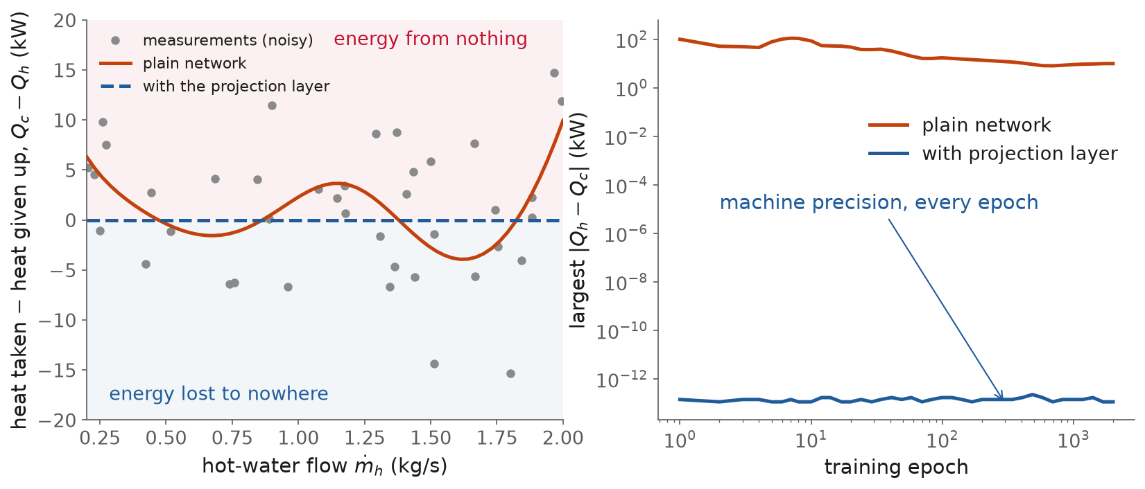
Fig. 101 The energy imbalance of each network’s predictions after 2,000 epochs (left), and the largest imbalance during training (right).

After 2,000 epochs	Without the layer	With the layer
Largest energy imbalance \(\lvert Q_c - Q_h \rvert\) on test flows	9.95 kW	\(1.1 \times 10^{-13}\) kW
Error in the outlet temperatures (RMSE)	0.49 °C	0.33 °C

• The layer holds the balance at every epoch, not only at the end.

• It is also more accurate here: it removes the part of the noise that breaks the balance.

• A plain network that fits the data well still creates or destroys up to 10 kW.

In the literature:

• KKT-hPINN (Chen, Constante Flores and Li, 2024) “rigorously guarantees hard linear equality constraints through projection layers derived from KKT conditions”. KKT stands for the Karush-Kuhn-Tucker conditions, the optimality conditions of a constrained problem. It was tested on Aspen models of a CSTR, an extractive distillation and a chemical plant (arXiv).

• KKT-Hardnet (Iftakher, Golder, Roy and Hasan, 2025) “enforces linear and nonlinear equality and inequality constraints up to machine precision”, by solving the KKT conditions of a distance minimization (arXiv).

• HardNet (Min and Azizan, 2024) appends “a differentiable closed-form enforcement layer to the network’s output”, and keeps the network a universal approximator (arXiv).

• Climate models (Beucler and colleagues, 2021): “architectural constraints enforce conservation laws to within machine precision without degrading performance” (arXiv).

Four approaches side by side

	PINN	Neural ODE	Neural DAE	Projection layer
Formulation	\(\min L_\text{data} + \lambda\lVert r\rVert^2\)	\(\dot x = f(x, \mathrm{NN})\)	\(\min L_\text{data}\) s.t. \(\dot x = f\), \(h = 0\), \(g \le 0\)	\(y = P(\mathrm{NN}(u))\)
Physics lives in	the loss	the right-hand side	the constraints of one NLP	the last layer
Physics held	favored, not enforced	balances held; bounds not	enforced, training and prediction	enforced, linear balances (nonlinear ones in new work, KKT-Hardnet)
Learns	one solution \(x(t)\)	the vector field	the unknown terms	a static map
Trained with	Adam	unconstrained solver + Adam (sequential)	nonlinear constrained optimization solver (simultaneous)	Adam

The same four, written as the optimization problem each one solves. The data-fit term is the same every time; what changes is where the physics sits, and so what the solver has to handle.

\[ \text{PINN:}\quad \min_{\theta}\; \sum_i \big(x_\text{NN}(t_i;\theta) - \hat x_i\big)^2 + \lambda \sum_j r\big(x_\text{NN}(t_j;\theta)\big)^2 \]

\[\begin{split} \begin{aligned} \text{Neural ODE:}\quad & \min_{\theta}\; \sum_i \big(x(t_i;\theta) - \hat x_i\big)^2 \\ & x(\cdot\,;\theta) = \mathrm{ODESolve}\big(f(x, \mathrm{NN}(x;\theta)),\, x_0\big) \end{aligned} \end{split}\]

\[\begin{split} \begin{aligned} \text{Neural DAE:}\quad & \min_{\theta,\,x,\,z}\; \sum_i \big(x(t_i) - \hat x_i\big)^2 \\ & \text{s.t.}\;\; \dot x = f(x, z),\;\; 0 = h(x, z),\;\; g(x, z) \le 0,\;\; z = \mathrm{NN}(x;\theta) \end{aligned} \end{split}\]

\[\begin{split} \begin{aligned} \text{Projection layer:}\quad & \min_{\theta}\; \sum_i \big(y(u_i;\theta) - \hat y_i\big)^2 \\ & y(u;\theta) = \arg\min_{y}\,\lVert y - \mathrm{NN}(u;\theta)\rVert^2 \;\;\text{s.t.}\;\; Ay = b \end{aligned} \end{split}\]

• PINN: the variables are the weights; no constraints; the physics is one more term to make small.

• Neural ODE: the variables are the weights; the ODE is solved inside the objective, so the balances hold at every iterate, and bounds are not in the problem.

• Neural DAE: the variables are the weights and every state at every collocation point; the equations and bounds are constraints, held at the solution to solver tolerance.

• Projection layer: the variables are the weights; the layer solves a small problem in closed form, so every output satisfies \(Ay = b\).

Not only neural networks

Every learned term in this session was a neural network. The physics-based formulations do not need one: the unknown term can be any model that fits data.

• Gaussian processes. In a hybrid model of a fed-batch culture, a Gaussian process (GP) regression model, which also reports its uncertainty, is the unknown right-hand side: “a coupling of polynomial regression with Gaussian Process Models as representation of the right-hand side of the ordinary differential equation system”, shown on “a typical fed-batch cultivation for monoclonal antibody production” (Cruz-Bournazou et al., 2022). Raissi and Karniadakis built GP priors around a known linear differential operator to “infer parameters of the linear equations from scarce and possibly noisy observations” (2017).

• Sparse regression. SINDy (sparse identification of nonlinear dynamics) learns the equation itself: from a library of candidate terms (\(1, x, y, x^2, xy, \dots\)) it keeps “the fewest terms in the dynamic governing equations required to accurately represent the data” (Brunton, Proctor and Kutz, 2016).

• Symbolic regression. A search over formulas returns a closed-form expression a person can read, such as \(\mu_{max} S / (K + S)\). PySR’s search is “a multi-population evolutionary algorithm” (Cranmer, 2023).

• Tree ensembles. In a hybrid model of a monoclonal antibody process, “while maintaining the mass balance of the mechanistic model, coefficients of the equations were estimated with random forest regression” (Nemoto et al., 2025). Trained gradient-boosted trees can also be written into a mixed-integer optimization model and optimized over (Mistry et al., 2021); one of their test cases is concrete mixture design. OMLT, the tool SiNDAE uses to put networks into Pyomo, embeds trees as well.

Limitations and trade-offs

PINNs

• The physics is a penalty: the residual is small, not zero, and depends on \(\lambda\).

• Training can fail on stiff problems, such as stiff chemical kinetics (Ji et al., 2021), and on solutions with high-frequency or multiscale features (Wang, Wang and Perdikaris, 2021).

• A plain PINN learns one solution: a new initial condition or parameter means training again, unless it is an input of the network.

• Use one when you know the equation, have few data, and can live with an approximate residual.

Neural ODEs, trained sequentially

• The differential equations hold, but bounds and algebraic constraints do not, unless you add penalties.

• Oscillating or unstable dynamics give local minima, as in the spring-mass.

• They scale well: mini-batches and GPUs. Use them for large data sets and large networks.

Neural DAEs, trained simultaneously

• The NLP grows with the network and the number of trajectories, so the simultaneous approach suits small and medium networks.

• The network needs smooth activations, and the time grid is fixed before solving.

• Feasible is not accurate: constraints keep the prediction physical, not correct.

• Use them when constraints must hold exactly: safety limits, regulated quality, mass balances, DAEs.

Projection layers

• They constrain one prediction at a time, not a trajectory over time.

• Linear equalities are cheap; inequalities and nonlinear constraints need a solve in every forward pass.

All hybrid models

• The mechanistic part must be right. If a balance is wrong, the network compensates in ways that do not transfer to new conditions.

• Physics constrains only what it describes. A learned term can still be wrong far from the data; the constraints only stop it from being impossible.

Worked examples

The code of this session, in order, with the data and the plots:

• l13-pinn-jax.ipynb: the spring-mass PINN from scratch in JAX: a plain network and a PINN with the same weights and steps, their extrapolation errors, and the residual that does not reach zero.

• l13-neural-dae.ipynb: the fed-batch bioreactor as a neural ODE in Diffrax, trained sequentially, then as a neural DAE in SiNDAE, following the SiNDAE fed-batch example; a new batch predicted by both, and the hours with negative substrate.

Summary

• Scientific machine learning keeps the mechanistic model and learns only the unknown term.

• A PINN puts the equation’s residual in the loss, evaluated at collocation points. It extrapolates far better than a plain network (0.001 m against 0.54 m here), but the physics is favored, not enforced: 5.3 N of residual is left.

• A recurrent network is the forward Euler discretization of a neural ODE. As the time step goes to zero, the steps converge to the ODE’s solution. A neural ODE learns the vector field, and a differentiable solver gives its gradients.

• A neural ODE of the bioreactor, trained sequentially, fits three batches and predicts −0.37 g/L of substrate on a new one. A purely data-driven model does worse: −0.43 g/L, and a biomass error of 0.43 g/L.

• Some physics must be enforced: balances, safety limits, bounds. Path constraints and DAEs hold at every instant.

• The sequential approach simulates at every iterate. The simultaneous approach discretizes and solves one NLP, satisfying the model only at convergence, but handling constraints and oscillating dynamics.

• A neural DAE trained and solved simultaneously (SiNDAE) keeps the substrate at or above zero on the new batch.

• Projection layers build linear constraints into the network itself, one prediction at a time: the heat exchanger’s energy balance held to \(10^{-13}\) kW.

• The learned term need not be a neural network: Gaussian processes, sparse and symbolic regression, and tree ensembles fill the same role.

Resources

• Raissi, Perdikaris and Karniadakis (2019), physics-informed neural networks. The paper that introduced PINNs.

• Ben Moseley, “So, what is a physics-informed neural network?”. The spring-mass PINN, explained with animations and PyTorch code.

• Krishnapriyan et al. (2021), failure modes of PINNs. Why PINNs fail on problems that look easy.

• Chen et al. (2018), Neural Ordinary Differential Equations. The Euler-step view of residual and recurrent networks.

• Kidger (2021), On Neural Differential Equations. A full, readable textbook on neural ODEs, CDEs and SDEs, with practical advice.

• Diffrax documentation. Differentiable ODE solvers in JAX.

• Rackauckas et al. (2020), Universal Differential Equations. Mechanistic models with a network for the unknown term.

• Biegler (2017), advanced optimization strategies for dynamic process operations. Sequential and simultaneous dynamic optimization, with path constraints on real reactors.

• Lueg et al. (2026), training neural DAEs with the simultaneous approach. The method behind SiNDAE, with the tank manifold, predator-prey and bioreactor studies. Open access.

• SiNDAE documentation. Quickstart and worked examples, including the fed-batch bioreactor.

• Reusch and Tejada (2015), Fc glycans as critical quality attributes. Why glycosylation matters for the safety and efficacy of antibody drugs. Open access.

• Chen, Constante Flores and Li (2024), KKT-hPINN. Projection layers for exact mass balances in chemical process models.

• Iftakher et al. (2025), KKT-Hardnet. Projection onto nonlinear equality and inequality constraints.

• Deep Implicit Layers tutorial. Neural ODEs, with code.

• Bradley et al. (2022), integrating first-principles and data-driven models. A review of hybrid modeling for process engineering (author’s copy).

Assignment

No assignment is released today.

Practice module

Practice module for this session, for participation credit.