Lecture 14: Uncertainty quantification in machine learning

At a glance

• Session Lecture 14, Week 7

• Arc Machine learning and deep learning

• Slides Deck for this session

• Practice Practice module for this session

• Demo l14-uq.ipynb, an ensemble, its recalibration, split conformal and CV+ on the concrete strength dataset, then four pycse regressors inside and beyond their data

• Tools scikit-learn for the Gaussian process and the networks, MAPIE for conformal prediction, pycse for models with uncertainty built in

Why this matters

Intervals that held, until the chemistry changed

A neural-network force field predicts the energy of a molecule or a surface from the positions of its atoms, in a fraction of the time a density functional theory (DFT) calculation takes. It is only useful if you know when to trust it, because the reason to use it is to avoid running DFT. So a force field needs an uncertainty attached to every prediction, and that uncertainty has to be right on the structures you have not computed.

Hu, Musielewicz, Ulissi and Medford (2022), with CMU Chemical Engineering co-authors, built exactly that. They combined conformal prediction, a method this session covers, with distances in the network’s internal representation, and put intervals on energies from neural-network force fields:

• On test data drawn like the training data, the intervals were calibrated and sharp.

• Calibrating them took minutes, against roughly 11,000 GPU-hours to train the underlying GemNet-OC model.

• Then they changed the chemistry. Trained on QM9 molecules without fluorine and tested on molecules with it, the 90% intervals covered 26% of the test molecules.

Nothing in the method was broken. Its guarantee rests on one condition, that the test structures resemble the calibration structures, and a molecule containing an element the model never saw does not. The intervals were as confident on the new chemistry as on the old, and wrong on most of it, and new chemistry is often why such a model is run.

Why this is a machine learning problem

The same problem appears in every surrogate model you train in this course. A network trained on 800 concrete mixes, a Gaussian process (GP) fitted to 40 simulation runs, a soft sensor trained on a quiet month of plant data: each returns a number for any input you give it, including inputs nothing like its training data. The number arrives with the same confidence either way unless the model also says how unsure it is.

Uncertainty quantification (UQ) is the practice of attaching that statement to a prediction and then checking it. This session covers both halves, with numbers you can reproduce from figures/make_figures.py:

• A GP fitted to five points, with its settings chosen by maximum likelihood, puts the truth inside its 95% band only 78% of the time (the median over 200 data sets).

• An ensemble of five networks on the concrete strength dataset covers 79% of test mixes at a nominal 90%. One number fitted on held-out mixes brings it to 90%.

• Split conformal prediction comes with a finite-sample guarantee of 90%. On the strongest mixes, held out from training, it covers 56%.

The order matters. We first define what is being claimed, then build the check, and only then look at methods, so that every method meets the same test.

Learning objectives

By the end of this session you should be able to:

• Define uncertainty quantification, distinguish aleatoric from epistemic uncertainty, and tell confidence, credible and prediction intervals apart.

• Check whether a predictive uncertainty is calibrated, with coverage, a reliability diagram and a proper scoring rule, and recalibrate it with one scale factor.

• Explain what a Gaussian process’s band promises, and recognize three ways it fails: heteroscedastic noise, a misspecified kernel, and too few data.

• Explain what the spread of a bootstrap or a deep ensemble measures, and why it needs a noise term and recalibration before it is an interval.

• Wrap any model in split conformal or CV+ prediction intervals, and state the exchangeability condition their guarantee rests on.

• Fit and compare UQ-capable regressors from pycse on data inside and beyond the training range.

What uncertainty quantification is

Definition: uncertainty quantification

Uncertainty quantification attaches to each prediction a distribution or an interval, together with a claim about how often the truth falls inside it.

The second half of that definition is what makes UQ testable. “The strength is 42 ± 6 MPa” says nothing until you add “and intervals stated this way contain the measured strength 90% of the time”. The rest of this session is about producing that claim and checking it.

Aleatoric and epistemic uncertainty

Definition: aleatoric and epistemic uncertainty

Aleatoric uncertainty is the scatter in the data itself, which more data does not remove. Epistemic uncertainty is what the model does not know yet, which more data in the right place reduces.

The terms come from engineering reliability analysis. Der Kiureghian and Ditlevsen give the practical test: uncertainty is epistemic if the modeler “sees a possibility to reduce” it by gathering data or refining the model (Structural Safety, 2009; paywalled, the DTU record has the abstract). Hüllermeier and Waegeman (2021) carry the split into machine learning, as reducible against irreducible uncertainty.

Move the sliders below. The noise sets a floor that no number of points lowers. The model’s own uncertainty shrinks where points arrive and grows back to the prior where they do not.

One detail surprises people: the split depends on the model. Hüllermeier and Waegeman (sec. 2.3) point out that adding an input feature can turn aleatoric uncertainty into epistemic. Concrete strength scatters at fixed mix proportions partly because curing temperature varies. To a model without temperature as an input, that scatter is noise. To a model with it, the same scatter is something the model can learn.

Where else uncertainty comes from

Noise and missing data are not the whole list. Kennedy and O’Hagan (2001) (a reading-group copy of the paper) list six sources for predictions made with a computer model: parameter uncertainty, model inadequacy, residual variability, parametric variability, observation error and code uncertainty. Two matter most for a surrogate:

• Model inadequacy: “No model is perfect.” Even with every input known, the model and reality differ. A wrong functional form is a model inadequacy, and no amount of data inside the training range reveals how wrong it is outside.

• Code uncertainty: the simulator is too expensive to run everywhere, so its output between runs is unknown. An ML surrogate of a simulator exists to manage exactly this.

Three kinds of interval

Three intervals get written as “± something”, and they answer different questions:

Interval	Covers	Interpretation
Confidence interval	the true function value \(f(x)\)	frequentist: the procedure covers in repeated use
Credible interval	the true function value \(f(x)\)	Bayesian: the posterior probability of the interval
Prediction interval	a new measurement \(y = f(x) + \varepsilon\)	either school; includes the noise

Heskes (1997) sets out the first and third for neural networks, and notes that “a prediction interval necessarily encloses the corresponding confidence interval”, because a new measurement carries the noise as well. Gelman et al., Bayesian Data Analysis (sec. 1.1, free PDF) explain the second: a Bayesian interval “can be directly regarded as having a high probability of containing the unknown quantity”, whereas a confidence interval refers to “a sequence of similar inferences”.

An engineer deciding whether a mix will pass a 40 MPa specification needs the prediction interval, because the specimen that gets tested is a new measurement. Every coverage number in this session is for prediction intervals.

Why machine learning makes this hard

A network trained by least squares returns one number. Uncertainty has to be added on, and the ways of adding it run into four problems:

• Training residuals are too small. A flexible model fits its training set more closely than it will fit new data, so a noise level estimated from training residuals is biased low. Laves et al. (2020) show that the maximum likelihood solution “systematically underestimates σ²”.

• Large networks are overconfident. Guo et al. (2017) found that a 110-layer ResNet’s confidence was “substantially higher than its accuracy”, while a small LeNet’s matched. Their study was of classification.

• ReLU networks extrapolate linearly. Hein et al. (2019) prove that a ReLU classifier becomes arbitrarily confident far from the data (their Theorem 3.1). For regression the same piecewise-linear structure means the prediction runs off in a straight line, with nothing in the model that grows its uncertainty.

• Nothing in the training data describes the region without data. Any statement about uncertainty there comes from an assumption: a prior, the diversity of an ensemble, or the assumption that test points resemble calibration points. The methods below differ mainly in which assumption they make.

Calibration: checking an uncertainty

The check comes before the methods because every method below claims to be right, and the only way to tell is to compare its intervals with held-out measurements.

Definition: calibration

An uncertainty is calibrated when its stated probabilities match what happens: 90% intervals contain the measured value 90% of the time.

Kuleshov et al. (2018) give the regression version: for every level \(p\), the fraction of test points below the predicted \(p\)-quantile should be \(p\) (their Eq. 3). In practice you check a handful of central intervals:

• Coverage at a level is the fraction of held-out points whose interval contains the measured value.

• A reliability diagram plots observed coverage against nominal coverage at several levels. On the diagonal: calibrated. Below it: overconfident, the intervals are too narrow. Above: underconfident.

Sharpness subject to calibration

Definition: sharpness

Sharpness is how narrow the predictive distributions are. It is a property of the forecasts alone, measured without looking at the outcomes.

Coverage alone can be gamed. An interval from 0 to 100 MPa covers every concrete specimen ever cast. Gneiting, Balabdaoui and Raftery (2007) (author’s copy) state the goal as “maximizing the sharpness of the predictive distributions subject to calibration”. Their example of what goes wrong without the second half is the climatological forecaster: it ignores the inputs and issues the long-run distribution of the outcome every time. It is perfectly calibrated and useless.

The concrete strength dataset has its own climatological forecaster: take the 5% and 95% quantiles of all training strengths and issue that interval for every mix. On held-out mixes it covers 91% at a nominal 90%, and its interval is 55.9 MPa wide. The recalibrated ensemble later in these notes covers 90% with intervals 22.2 MPa wide. Both are calibrated. Only one is useful.

Proper scoring rules

A single number that rewards calibration and sharpness together is a proper scoring rule: a score whose expected value is best when the forecast distribution equals the true one, so it cannot be improved by hedging (Gneiting and Raftery, 2007, author’s copy). Two are standard for regression:

• Negative log likelihood (NLL): for a Gaussian prediction with mean \(\mu\) and standard deviation \(\sigma\), \(\tfrac{1}{2}\log(2\pi\sigma^2) + \tfrac{(y-\mu)^2}{2\sigma^2}\), averaged over test points. It punishes a confident miss heavily, because \(\sigma\) appears in the denominator. Gneiting and Raftery note that this unboundedness makes it sensitive to a few bad points.

• Continuous ranked probability score (CRPS): the squared distance between the predicted cumulative distribution and a step at the observed value. Gneiting and Raftery note that it “generalizes the absolute error”, to which it reduces for a point forecast, so it carries the units of \(y\).

Lower is better for both. Report one of them alongside coverage and width.

Calibrated on average is not calibrated everywhere

A model can hit 90% overall by over-covering easy points and under-covering hard ones. Levi et al. (2022) argue that Kuleshov’s definition “has severe limitations in distinguishing informative from non-informative uncertainty predictions”, and propose binning test points by predicted \(\sigma\) and comparing the root mean square error with the mean \(\sigma\) in each bin. Pernot (2023) names two stronger properties:

• Consistency: calibration conditional on the predicted uncertainty. Points the model calls uncertain should have large errors.

• Adaptivity: calibration conditional on the input. The intervals should be right in every region of input space.

Pernot shows that good consistency “does not imply a good adaptivity”. Checking coverage separately on a held-out region of input space, as the extrapolation split below does, is an adaptivity check.

Recalibration, and where it stops working

If a model’s intervals are consistently too narrow, you can widen them after training using held-out data. Two common forms:

• Scaling: multiply every \(\sigma\) by one factor \(s\) fitted on held-out data. This is σ scaling (Laves et al., 2020) or STD scaling (Levi et al., 2022). The ensembles section below works it through.

• Isotonic recalibration: fit a monotone map from predicted to observed cumulative probability (Kuleshov et al., 2018, Algorithm 1).

Both learn a correction from held-out data, so both inherit the assumption that future data resemble that held-out data. Kuleshov’s guarantee needs “enough i.i.d. data”, and the paper notes that a recalibrated quantile degrades under “a shift in the data distribution”. Ovadia et al. (2019) measured this for classifiers: the error of temperature scaling “increases significantly as the shift increases”. A correction learned on one region of input space does not carry to another.

Case study: comparing UQ methods for catalysis

Tran et al. (2020), from Ulissi’s group at CMU Chemical Engineering, compared UQ methods for density functional theory (DFT) adsorption energies using calibration curves, the area between the curve and the diagonal, sharpness, and NLL. It is a model for how to report a UQ comparison: several metrics together, since each can be gamed on its own.

Gaussian processes

A GP is the method where uncertainty is part of the model rather than added afterwards, which makes it the natural place to start, and the clearest place to see what an uncertainty rests on.

Definition: Gaussian process

A Gaussian process is a probability distribution over functions, set by a kernel that says how strongly the function’s values at two inputs are correlated.

Prior and posterior

Before any data, the kernel defines a prior: a spread of smooth functions centered on zero. Conditioning on observations gives the posterior: the functions from the prior that pass near the data (Rasmussen and Williams, 2006, ch. 2, free from the authors).

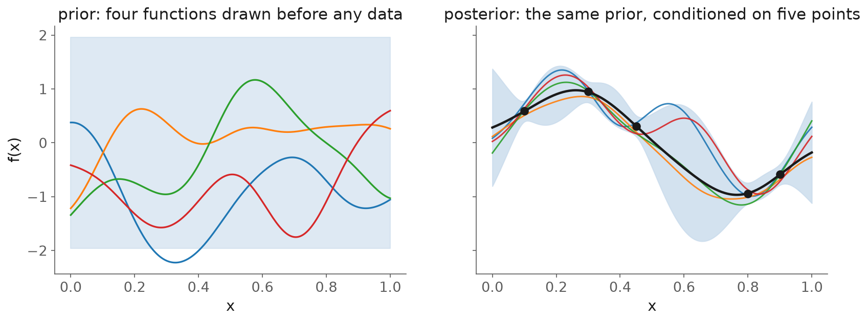
Fig. 102 Left: four draws from a GP prior with an RBF kernel of length scale 0.15. Right: the same prior conditioned on five points of \(\sin(2\pi x)\). After Rasmussen and Williams, Fig. 2.2.

With training inputs \(X\), targets \(y\), kernel matrix \(K = k(X, X)\), noise variance \(\sigma_n^2\) and the vector \(k_*\) of kernel values between a new input \(x_*\) and the training inputs, the predictive mean and variance are (Rasmussen and Williams, Eqs. 2.25 and 2.26):

\[ \mu(x_*) = k_*^\top (K + \sigma_n^2 I)^{-1} y, \qquad \sigma^2(x_*) = k(x_*, x_*) - k_*^\top (K + \sigma_n^2 I)^{-1} k_* \]

Two consequences follow from the variance formula:

• Far from the data, \(k_*\) goes to zero and the variance returns to the prior variance. Rasmussen and Williams: “the error bars reflect the prior standard deviation of the process \(\sigma_f\) away from the data” (p. 20).

• The variance does not contain \(y\). It depends “only on the inputs” (p. 18). At fixed kernel settings, a GP that fits the data badly reports exactly the same band as one that fits it well. Deringer et al. (2021) add the refinement: once the kernel settings are fitted to the data, the variance does “implicitly depend on training function values”. So the band reacts to a bad fit only through the hyperparameters.

Choosing the settings by maximum likelihood

The kernel has settings: a length scale (how far apart two inputs can be and still be correlated), a signal standard deviation \(\sigma_f\), and the noise standard deviation \(\sigma_n\). scikit-learn chooses them by maximizing the log marginal likelihood, the probability of the observed \(y\) under the GP (Rasmussen and Williams, Eq. 2.30).

Try it below on a smooth function sampled at 12 points with noise of standard deviation 0.1. Press “Fit”. Then click the plot to add points, and fit again.

With these 12 points, maximum likelihood sets the noise to 0.044, less than half the true 0.1, and the 95% band covers only 66% of new observations in \([0, 1]\). Beyond the data, the band widens to the prior and covers 96%. The GP is overconfident where it has data and honest where it has none, the opposite of the usual worry.

Failure 1: noise that grows with the input

A standard GP has one noise level, \(\sigma_n\), for every input: Rasmussen and Williams’ Eq. 2.20 assumes “independent identically distributed Gaussian noise”. In engineering data the noise often grows with the signal: a flow meter with a percentage-of-reading error, a strength test whose scatter grows with strength.

The toy problem below has noise of standard deviation \(0.02 + 0.3x\), so it is 16 times larger at \(x = 1\) than at \(x = 0\). Fitted to 60 points, the GP chooses one noise level of 0.20. Coverage over the whole range is a respectable 95%, but by third of the range it is 100%, 98% and 88%: too wide on the left, too narrow on the right. The average hides both errors.

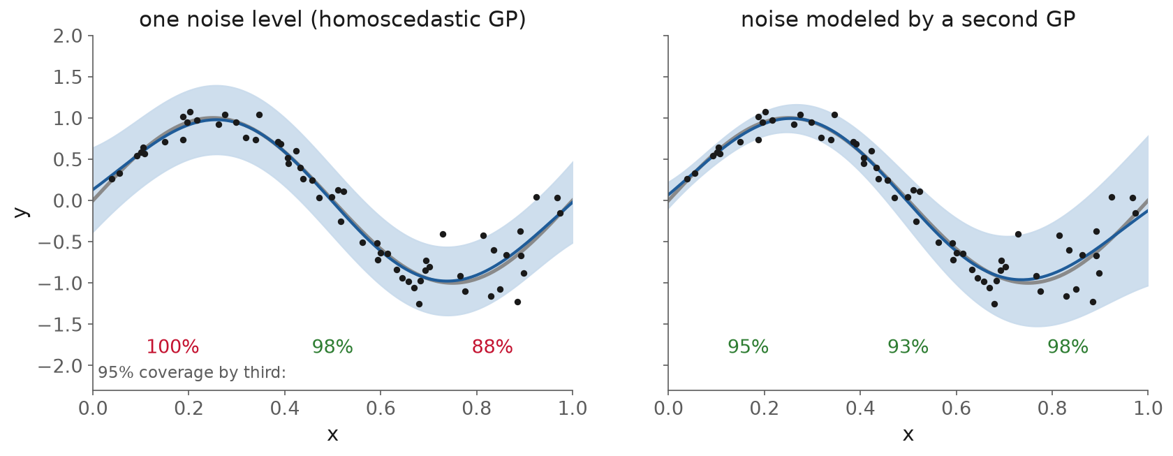
Fig. 103 95% coverage by third of \([0, 1]\), exact against the known truth and noise. Left: one noise level. Right: the noise level learned per point.

The standard fixes model the noise level as a function of the input:

• Goldberg, Williams and Bishop (1998) put a second GP on the log of the noise level, so the noise varies smoothly with the input.

• Kersting et al. (2007) use a cheap alternation instead: fit a GP, estimate the noise at each training point from its residuals, fit a second GP to those estimates, refit the first with that noise, and repeat.

• Lázaro-Gredilla and Titsias (2011) give a variational version. They call constant noise “too restrictive … but one that is needed for GP inference to be tractable”, and their method costs about twice a standard GP.

The right panel uses a simplified version of Kersting’s alternation, and building it turned up a surprise. The first version learned a noise level about 0.7 times too small everywhere. The reason is a bias in the log of a squared residual: for Gaussian noise, \(\mathbb{E}[\log \varepsilon^2] = \log \sigma^2 - 1.27\), so regressing \(\log r^2\) on \(x\) estimates the log variance 1.27 too low. Adding 1.27 back recovered the noise level and gave coverage of 95%, 93% and 98% by third.

Common pitfall: a per-point alpha is not a heteroscedastic GP

scikit-learn’s GaussianProcessRegressor accepts an array for alpha, one noise variance per training point. That changes how the GP weighs the training data. It does not give the GP a noise model, so predict(..., return_std=True) at a new input still returns no noise term for that input, and a WhiteKernel estimates “the global noise level” (scikit-learn user guide). To predict with input-dependent noise, you need a model of the noise at the new input, as above.

Failure 2: a kernel that does not match the function

The RBF kernel assumes the function is smooth everywhere, with one length scale. A function with a step violates that assumption. Fitted to 40 points of a function with a jump at \(x = 0.5\), the GP covers 98% of the range away from the step and 72% within 0.1 of it.

The fitted length scale carries a warning sign. To bend sharply at the step, the GP shortens its length scale everywhere, and with more data it keeps shortening. Duvenaud’s kernel cookbook calls a length scale that “never stops becoming smaller as you add more data” “a classic sign of model misspecification”. The figure shows it happening.

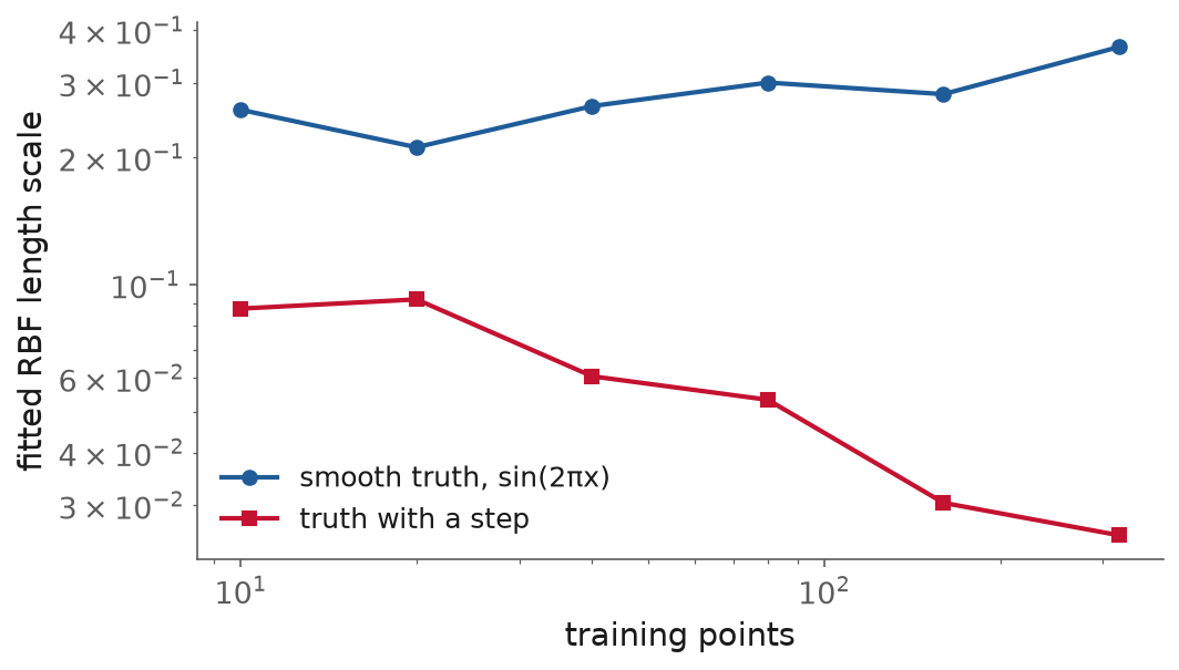
Fig. 104 Fitted length scale against the number of training points, median of five data sets each. Smooth truth: about 0.2 to 0.4 at every size. Truth with a step: from 0.088 at 10 points to 0.025 at 320.

The general point is that a GP’s band is calibrated only if the data look like draws from its prior. Capone, Pleiss and Hirche (2023) put it directly: GP uncertainties “can be miscalibrated in practice”, because “the distribution of unseen data seldom follows the Gaussian prior distribution”.

Failure 3: too few points

The third failure is the one that matters most for expensive experiments. With few points, many settings explain the data about equally well, and maximum likelihood picks one of them as if it were known. Capone, Lederer and Hirche (2022) describe the case where, with “little data”, “both short and long lengthscales explain the data consistently”, which leads to “overconfident error bounds”. Rasmussen and Williams show two local optima from seven points (sec. 5.4.1, Fig. 5.5).

To see how often this happens, make_figures.py fits a GP to 200 random data sets of each size from the same smooth function and noise, and computes the exact coverage of each 95% band:

Training points	Median coverage	Data sets below 80%	Data sets below 50%
5	78%	52%	26%
12	92%	21%	1%
40	95%	0%	0%

With five points, a quarter of the fitted GPs cover less than half of new observations with what they call 95% intervals. Fiedler, Scherer and Trimpe (2021) explain why no guarantee covers this case: GP error bars are Bayesian statements about the posterior, not frequentist guarantees, and the rigorous bounds that do exist are “too conservative” to be used, so practitioners fall back on heuristics, “thus breaking all theoretical guarantees”.

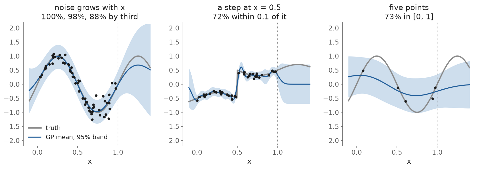
Fig. 105 The three failures side by side, with the exact 95% coverage that shows each one.

Cost and dimension

• Cost. Exact GP inference needs a solve with the \(n \times n\) kernel matrix, which costs \(O(n^3)\) time (Rasmussen and Williams, p. 6). Sparse approximations summarize the data with \(m\) inducing points and cut the cost “from \(O(n^3)\) to \(O(nm^2)\)” (Titsias, 2009; Snelson and Ghahramani, 2006).

• Dimension. In many dimensions distances between points become similar, and a stationary kernel has little to work with. Binois and Wycoff (2022) write that the GP prior “simply says too little when dimension grows too large”.

Case study: a materials GP that missed a minimum

Deringer et al. (2021), a review of GPs for materials and molecules (open access), discuss a GP interatomic potential for silicon (sec. 5.2, Fig. 24). Along a path toward a defect structure, the model’s predicted error “rises notably” where it departs from DFT, so the band widens where the model is wrong. But the GP potential also misses a minimum that DFT finds, and the review notes that the minimum “will not be revealed by simulations using this specific GAP model”. A model can flag that it is uncertain without telling you what it is missing.

What a practitioner should take from this

• Fit the noise and look at it. A fitted noise far below what replicate measurements show means the band is too narrow.

• Check coverage by region, not only overall. Heteroscedastic noise hides inside an average.

• Watch the fitted length scale as data arrive. If it keeps shrinking, the kernel is wrong.

• With fewer than about a dozen points, treat a GP’s band as a rough guide rather than a 95% statement.

Bootstrap and ensembles

The second family gets uncertainty from disagreement: train several models and use the spread of their predictions. It works with any model, which is why it is everywhere.

The bootstrap

Definition: bootstrap

The bootstrap resamples the training data with replacement, refits the model on each resample, and uses the spread of the refitted models as an estimate of how much the fit varies with the data.

Efron (1979) introduced the bootstrap to “estimate the sampling distribution of some prespecified random variable”. For a regression model, the spread across resamples estimates how much the fitted function would change if you collected a new data set of the same size. That is the variance part of the error. It misses two things:

• The noise. The spread is about the fitted function, not about a new measurement, so it is a confidence interval, not a prediction interval.

• The bias. If every resample leads to the same wrong answer, the spread is small and the error is large. Heskes (1997) states the assumption plainly: “the bias component of the confidence intervals is negligible in comparison with the variance component.” Palmer et al. (2022) warn that the bootstrap “may… fail entirely when bias is a dominant source of error”, as happens “far outside the domain of the model”.

Deep ensembles

Definition: deep ensemble

A deep ensemble trains several networks that differ only in their random starting weights and data order, and combines their predictions.

Lakshminarayanan, Pritzel and Blundell (2017) proposed two ingredients, and both matter:

• Different random starts, not resamples. “We observed that bagging deteriorated performance in our experiments”. Each network sees all the data. They used five networks.

• A noise term. Each network predicts a mean and a variance and is trained on the Gaussian NLL, so the ensemble’s predictive variance is the average predicted noise plus the spread of the means. The spread alone measures only the epistemic part.

Fort, Hu and Lakshminarayanan (2019) explain why random starts are enough: networks from different starts land in different modes of the loss surface, so they represent different functions.

What the spread measures

The widget below trains ten two-layer ReLU networks on 120 noisy points of \(\sin(2\pi x)\) on \([0, 1]\), either from different seeds or from bootstrap resamples, and asks about \([1, 1.5]\) as well. Coverage is exact against the known truth.

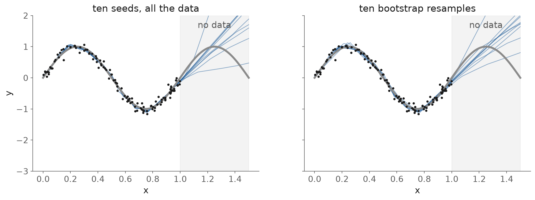
Fig. 106 Ten networks from different seeds (left) and from bootstrap resamples (right). Shaded: beyond the training data.

95% intervals	Inside the data	Beyond the data
Seeds, spread only	29%	85%
Seeds, spread plus a noise estimate	93%	93%
Bootstrap, spread only	52%	81%
Bootstrap, spread plus a noise estimate	94%	87%

Inside the data, the ten seeded networks agree to within 0.021 on average, while the noise has a standard deviation of 0.1. The spread is the epistemic part only, so an interval built from it alone covers 29%. Adding a noise estimate, here the standard deviation of the training residuals of the ensemble mean, brings it to 93%.

Beyond the data, in this example, the members fan out: their spread averages 0.63 against an error of 0.61, and coverage stays near 90%. Nothing guarantees this. In one dimension, with nothing beyond \(x = 1\) to constrain them, the networks have every reason to disagree. The published evidence on real problems is mixed, and the next section collects it.

The evidence on ensembles

Ensembles are the strongest widely available baseline, and they are not calibrated out of the box. Both statements are well supported.

• The strongest baseline. Ovadia et al. (2019) compared methods under dataset shift and concluded that “deep ensembles seem to perform the best across most metrics and be more robust to dataset shift”. They also found that uncertainty quality “consistently degrades with increasing dataset shift regardless of method”. Their benchmarks were classification.

• In chemistry. Scalia et al. (2020) and Tan et al. (2023) found ensembles at or near the top for molecular properties and interatomic potentials. Tan et al. conclude that “single deterministic models cannot yet consistently match or outperform ensembling”.

• Overconfident in level. Hirschfeld et al. (2020) report that “traditional ensembling consistently underestimates uncertainty”. Kahle and Zipoli (2022) find interatomic-potential ensembles “often overconfident” and say they “require to be calibrated for each system and architecture”. Palmer et al. found the opposite direction for random-forest bootstrap ensembles in domain, which over-estimate; either way a correction is needed.

• Weakest where it matters most. On scaffold splits, where test molecules differ structurally from training ones, Scalia et al. found coverage “always underestimated”, “particularly affecting high-error predictions”.

• Cost. \(M\) networks cost \(M\) times as much to train and to evaluate.

So an ensemble’s spread is a useful relative signal of where the model is unsure. It is not an interval until it has a noise term and has been checked against held-out data, and usually rescaled.

Worked example: recalibrating an ensemble

This example uses the concrete strength dataset from Lecture 9, with Lecture 9’s network (one hidden layer of 16 tanh units) and two test sets:

• Grouped split: 20% of the mixes held out at random (195 test rows), as in Lecture 9.

• Extrapolation split: the 20% of mixes with the lowest water/cement ratio held out (265 test rows). These are the strongest mixes, and a design loop pushes a surrogate exactly there.

Within each training set, a quarter of the mixes are set aside as calibration mixes (210 and 213 rows), and five networks with seeds 0 to 4 are trained on the rest. The interval for a test mix is the ensemble mean \(\pm z \cdot s \cdot \sigma_{\text{ens}}\), where \(\sigma_{\text{ens}}\) is the spread and \(s\) is one scale factor.

Fitting \(s\). For calibration mixes \(i = 1, \dots, n\), write \(z_i = (y_i - \mu_i)/\sigma_i\). The Gaussian NLL of the rescaled predictions is, up to a constant,

\[ \text{NLL}(s) = \frac{1}{n}\sum_{i=1}^n \left[ \log(s\,\sigma_i) + \frac{z_i^2}{2 s^2} \right]. \]

Setting its derivative \(1/s - \overline{z^2}/s^3\) to zero gives

\[ s^2 = \frac{1}{n}\sum_{i=1}^n z_i^2 , \]

the mean square of the calibration \(z\)-scores. A calibrated model has \(z\)-scores with unit variance, so \(s\) measures how far from that the model is. The same one-parameter correction has been published at least four times: σ scaling (Laves et al.), STD scaling (Levi et al.), the calibrated committee of Musil et al. (2019), and Eq. 8 of Kellner and Ceriotti (2024).

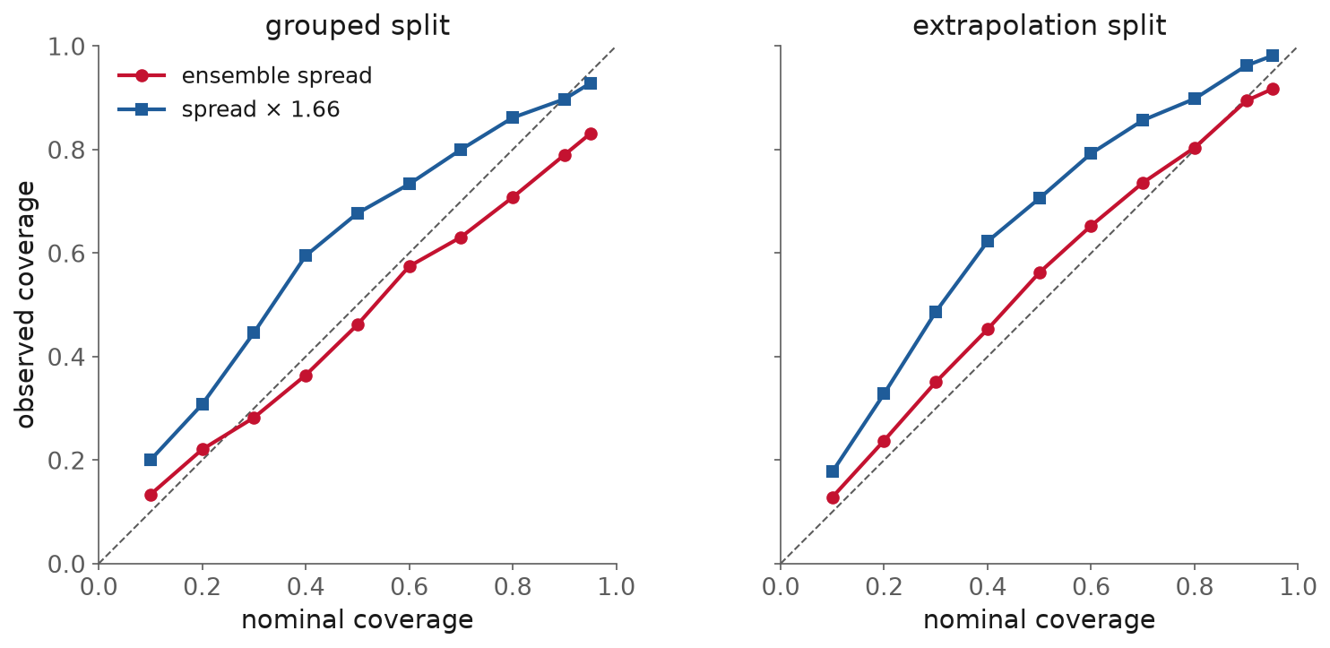
Fig. 107 Reliability diagrams for the raw ensemble spread and for the spread rescaled by \(s\), fitted on each split’s calibration mixes.

90% intervals	Grouped: raw	Grouped: rescaled	Extrapolation: raw	Extrapolation: rescaled
Scale factor \(s\)	1	1.66	1	1.44
Coverage	79%	90%	89%	96%
Mean width (MPa)	13.4	22.2	35.3	50.9
NLL	3.72	3.22	3.74	3.81

On the grouped split the raw spread is overconfident, covering 79%. The factor fitted on the calibration mixes, \(s = 1.66\), brings test coverage to 90% and lowers the NLL from 3.72 to 3.22. Most of that factor is the missing noise: the spread measures disagreement between networks, while 19 settings in the dataset (the same mix at the same age) were tested more than once, and their strengths scatter with a pooled standard deviation of 5.0 MPa.

On the extrapolation split, the networks disagree much more (mean spread 10.7 MPa, against 4.1 on the grouped split), and the raw spread already covers 89%. Applying the factor fitted on the calibration mixes, which resemble the training mixes, over-widens the intervals to 96% and makes the NLL slightly worse. One number fitted in distribution does not transfer to a region it never saw, in either direction.

The spread is also a weak guide to which individual mixes will have large errors: the rank correlation between a test mix’s absolute error and its spread is 0.29 on the grouped split and 0.17 on the extrapolation split.

What a practitioner should take from this

• Never report an ensemble’s spread alone as an interval. Add a noise term, or rescale.

• Recalibration needs a third split of the data, separate from training and testing.

• Fit the scale factor on data that look like where the model will be used. If you cannot, report coverage on a held-out region and accept that it may be wrong in either direction.

Conformal prediction

The third family makes no assumption about the model at all. It takes any point predictor and sets the interval width from the errors the model makes on held-out data, with a guarantee that needs only one condition.

Definition: split conformal prediction

Split conformal prediction sets the width of a prediction interval from the model’s errors on a held-out calibration set, chosen so that the interval covers a new point with a stated probability.

The algorithm

The method grew out of Vovk, Gammerman and Shafer’s Algorithmic Learning in a Random World (2005). The split version, which needs one model fit, is due to Papadopoulos et al. (2002) and was analyzed for regression by Lei et al. (2018), from CMU Statistics. Angelopoulos and Bates give the clearest introduction.

1. Split the training data into a fitting set and a calibration set of \(n\) points.

2. Fit any model \(\hat\mu\) on the fitting set.

3. On the calibration set, compute the scores \(s_i = |y_i - \hat\mu(x_i)|\).

4. Let \(\hat q\) be the \(\lceil (n+1)(1-\alpha) \rceil\)-th smallest score.

5. The interval for a new input is \(\hat\mu(x) \pm \hat q\).

Definition: exchangeability

Data points are exchangeable when their joint distribution does not change if you reorder them: the calibration points and the test point were generated the same way.

The guarantee. If the calibration points and the new point are exchangeable, then

\[ 1 - \alpha \;\le\; P\big(y_{\text{new}} \in \hat\mu(x_{\text{new}}) \pm \hat q\big) \;\le\; 1 - \alpha + \frac{1}{n+1}, \]

for any model, any data distribution, and any finite \(n\) (Angelopoulos and Bates, Eq. 1 and Theorems D.1 and D.2; the upper bound needs scores without ties). No Gaussian assumption and no large-sample limit is involved.

Two details catch people:

• The quantile is slightly above \(1 - \alpha\). The \((n+1)\) accounts for the new point. With too few calibration points the required rank exceeds \(n\), and Lei et al. then set the interval to infinity. At \(\alpha = 0.1\) you need at least 9 calibration points.

• The probability is over the draw of the calibration set and the test point together. A particular calibration set can give coverage a little above or below \(1 - \alpha\).

Marginal coverage, not conditional coverage

The guarantee is marginal: averaged over all inputs. It says nothing about coverage at a particular \(x\), and Lei et al. (sec. 5.2) point out that for split conformal “the width is exactly constant over x”. On the toy problem above, where the noise grows from 0.05 to 0.3, the 90% band covers 92% overall, and by third of the range 100%, 95% and 82%.

Coverage at every \(x\) is not achievable without assumptions. Vovk (2012) showed that exact conditional validity “cannot be achieved in a useful way” when inputs are continuous, and Foygel Barber et al. (2021) proved that any method with distribution-free conditional coverage must produce intervals of infinite expected length almost everywhere (their Proposition 1).

Approximate fixes change the score so that the width follows the difficulty:

• Normalized scores: divide each residual by an estimate of its spread, \(|y - \hat\mu(x)| / \hat\rho(x)\), and the interval becomes \(\hat\mu(x) \pm \hat q\,\hat\rho(x)\) (Lei et al., sec. 5.2). On the toy problem, with \(\hat\rho\) a small network fitted to the absolute residuals, coverage by third becomes 94%, 91% and 90%.

• Conformalized quantile regression (CQR): fit quantile regressions for the lower and upper bounds, then conformalize their errors (Romano, Patterson and Candès, 2019). It is “fully adaptive to heteroscedasticity”, and its guarantee is still marginal.

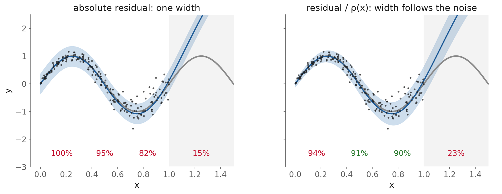
Fig. 108 90% split conformal on noise of standard deviation \(0.05 + 0.25x\), with coverage by third of \([0, 1]\) and beyond it. Left: one width. Right: residuals divided by \(\hat\rho(x)\).

Jackknife+ and CV+

Split conformal spends part of the data on calibration. With small data, that hurts the model. The jackknife+ of Barber et al. (2021) uses every point for both jobs:

1. For each training point \(i\), fit the model without it, giving \(\hat\mu_{-i}\), and record the leave-one-out residual \(R_i = |y_i - \hat\mu_{-i}(x_i)|\).

2. For a new \(x\), collect \(\hat\mu_{-i}(x) - R_i\) and \(\hat\mu_{-i}(x) + R_i\) over all \(i\).

3. The interval runs from the \(\lfloor \alpha(n+1) \rfloor\)-th smallest of the first set to the \(\lceil (1-\alpha)(n+1) \rceil\)-th smallest of the second.

The leave-one-out predictions at the new point carry the model’s own variability into the interval. The “+” in the name refers to this step, and the coverage guarantee depends on it. CV+ does the same with \(K\) folds instead of \(n\) refits.

The guarantee is weaker on paper. The worst case is \(1 - 2\alpha\) (their Theorem 1), and Theorem 2 shows that the factor of 2 cannot be removed in general. The authors add that “in practice” the coverage is close to \(1 - \alpha\). The plain jackknife, without the “+”, has no guarantee, and its coverage “may actually vanish”. The cost is \(n\) or \(K\) model fits instead of one.

On the concrete data, with the five-network ensemble as the model and ten folds by mix:

90% intervals	Grouped: coverage	Grouped: width (MPa)	Extrapolation: coverage	Extrapolation: width (MPa)
Split conformal	94%	20.9	56%	13.9
Normalized by the ensemble spread	90%	22.0	95%	49.4
CV+	98%	23.0	74%	20.1
Climatology	91%	55.9	54%	43.7

On the grouped split, every conformal method meets its target, as the guarantee says it should.

Out of domain

On the extrapolation split, split conformal covers 56%. Its width was set on calibration mixes that look like the training mixes, and the strongest mixes are not exchangeable with them: they were held out precisely because they are different. The guarantee did not fail. Its condition was not met.

The toy widget shows the same thing as the test window slides out of the calibration range: 90% target, and coverage of 99%, 94%, 86%, 56% and 16% as the window moves from \([0, 0.5]\) to \([1, 1.5]\). Normalizing by the ensemble spread rescued the concrete extrapolation split (95%) because that spread happens to grow on those mixes. It is not a general fix: on the toy problem, where the residual model \(\hat\rho\) knows nothing beyond \(x = 1\), normalized scores reach only 23% there.

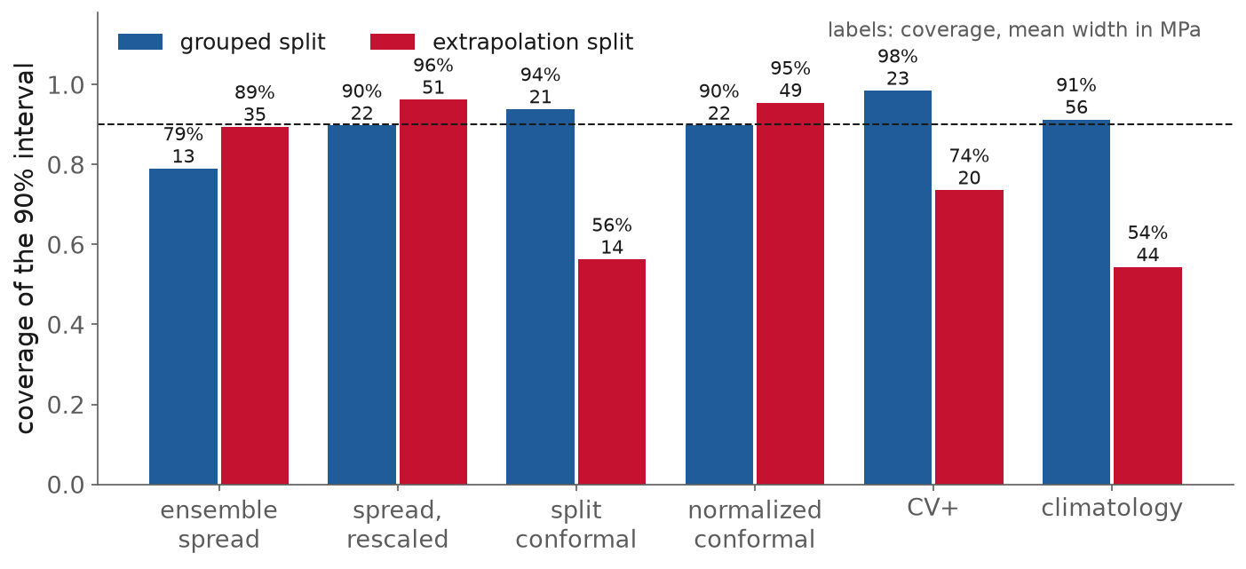
Fig. 109 Coverage of 90% intervals on the concrete strength dataset, with mean widths in MPa.

There are partial remedies when the shift is known:

• Weighted conformal prediction reweights the calibration scores by the likelihood ratio between test and training input distributions (Tibshirani et al., 2019). The ratio must be known or estimated, and their result assumes the test inputs lie where training inputs could also occur. So weighting can correct a change in emphasis, not true extrapolation.

• Barber et al. (2023) bound the coverage lost when exchangeability fails, in terms of distances between distributions that you usually cannot compute. The bound explains a loss rather than certifying coverage.

The fluorine case that opens these notes is this failure in a chemical engineering setting: intervals calibrated on molecules without fluorine covered 26% of molecules with it.

In code: MAPIE

MAPIE (Taquet et al., 2022) implements these methods for scikit-learn models. Version 1 renamed the classes: MapieRegressor became SplitConformalRegressor, CrossConformalRegressor and JackknifeAfterBootstrapRegressor, and alpha became confidence_level. Most tutorials online still use the old names.

from mapie.regression import SplitConformalRegressor, CrossConformalRegressor

# model already fitted on the fitting set
split = SplitConformalRegressor(model, confidence_level=0.9, prefit=True)
split.conformalize(X_cal, y_cal)
y_pred, y_int = split.predict_interval(X_test)        # y_int[:, 0, 0], y_int[:, 1, 0]

cvplus = CrossConformalRegressor(model, confidence_level=0.9, method="plus", cv=GroupKFold(10))
cvplus.fit_conformalize(X_train, y_train, groups=groups_train)

The notebook runs both and checks them against the hand-written versions.

UQ built into models: pycse

The last family builds uncertainty into a network so that one model, trained once, returns a mean and a standard deviation. pycse collects several as scikit-learn-style regressors. They share an API, predict(X, return_std=True), and most share one idea: treat the last layer of a network as a linear model on learned features, and use the well-understood uncertainty of linear regression there.

The idea has a known weakness, stated in Bishop’s Pattern Recognition and Machine Learning (sec. 3.3.2, free PDF): with localized basis functions “the model becomes very confident in its predictions when extrapolating outside the region occupied by the basis functions”. Features learned by a network are often like that.

Four models, each a distinct idea:

• LinearRegressionUQ (pycse.sklearn.lr_uq): ordinary least squares with the standard prediction standard error, the noise variance \(s^2\) plus the parameter term \(x_*^\top (X^\top X)^{-1} x_*\, s^2\) (Bishop, Eq. 3.59, is the Bayesian form). It is the baseline: correct if the basis is right.

• NeuralNetworkBLR (pycse.sklearn.nnbr): fit a network, then a Bayesian linear regression on its last hidden layer. This is the “neural linear” model of Snoek et al. (2015), used there to scale Bayesian optimization.

• DPOSE (pycse.sklearn.dpose): a shallow ensemble, in which the networks share every layer except the last, trained so the spread of the last-layer outputs is itself fitted (Kellner and Ceriotti, 2024). The overhead is about one extra layer. predict_ensemble returns the members, so the uncertainty can be pushed through any derived quantity. The paper is candid that it is “generally overconfident for these extrapolative predictions”.

• LLPRRegressor (pycse.sklearn.llpr_regressor): last-layer prediction rigidity (Bigi et al., 2024). After ordinary training, the variance at a new input is \(\alpha^2 f_*^\top (F^\top F + \zeta^2 I)^{-1} f_*\), where \(F\) holds the last-layer features of the training data (their Eq. 25), with \(\alpha\) and \(\zeta\) fitted on validation data. It costs one forward pass.

Common pitfall: import from the module, not the package

In pycse 2.11.1, from pycse.sklearn import NNBR (and NNGMM, LLPR) raises ImportError. Import the classes from their modules: from pycse.sklearn.nnbr import NeuralNetworkBLR, from pycse.sklearn.llpr_regressor import LLPRRegressor.

make_figures.py fits all four, five seeds each, to 120 noisy points of \(\sin(2\pi x)\) on \([0, 1]\) (noise 0.1, plus 40 validation points), and computes the exact coverage of their 95% intervals inside the data and on \((1, 1.5]\):

95% intervals, mean of 5 seeds	Inside \([0, 1]\)	Width	Beyond, \((1, 1.5]\)	Width
LinearRegressionUQ (cubic basis)	94%	0.48	2%	0.87
NeuralNetworkBLR	95%	0.41	40% (15% to 69%)	1.38
DPOSE	93%	0.42	63% (46% to 73%)	1.26
LLPRRegressor	93%	0.43	84% (61% to 100%)	2.01

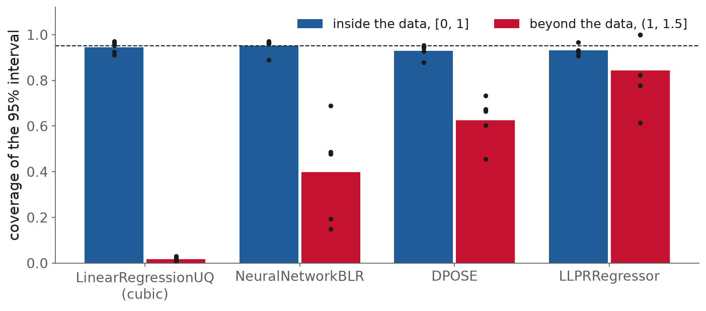
Fig. 110 Coverage of the 95% interval for four pycse regressors, five seeds each (dots), inside the training range and beyond it. Dashed: the nominal 95%.

Inside the training range all four are calibrated, at 93% to 95%. Beyond it, they separate:

• LinearRegressionUQ falls to 2%. Its band does widen, from 0.48 to 0.87, but the cubic basis is wrong for a sine, and the parameter term only measures uncertainty within that basis. The model inadequacy of Kennedy and O’Hagan is invisible to it.

• NeuralNetworkBLR covers 40% on average, and anywhere from 15% to 69% depending on the seed. Bishop’s warning about features describes it.

• DPOSE covers 63%, consistent with its authors’ own caveat about extrapolation.

• LLPRRegressor covers 84%, mostly by widening: its band beyond the data is 2.01 wide, nearly five times its width inside.

While fitting, NeuralNetworkBLR printed “✓ Model is well-calibrated” for every seed. The check behind that message rescales the band on the validation points, which come from \([0, 1]\), so it is an in-distribution statement, made about a model that went on to cover 40% beyond its data.

Limitations and trade-offs

Every method in this session is calibrated relative to an assumption, and each one fails when its assumption fails:

Method	Assumes	Guarantee	Beyond the data	Cost
Gaussian process	the function is a draw from the kernel’s prior; one noise level	Bayesian, conditional on the prior	band returns to the prior: honest if the prior is	\(O(n^3)\); struggles in high dimension
Ensemble spread	members disagree where they are wrong	none	sometimes fans out, sometimes agrees; needs checking	\(M\) trainings and \(M\) evaluations
Ensemble, rescaled	the calibration data resemble the use	none; empirical	the scale factor does not transfer	one extra data split
Split conformal	calibration and test points are exchangeable	finite-sample, marginal, any model	none; coverage falls	one extra data split
CV+	training and test points are exchangeable	marginal, at least \(1 - 2\alpha\)	none; coverage falls	\(K\) model fits
Last-layer models (pycse)	the learned features stay informative beyond the data	none	often overconfident	about one model

Some trade-offs cut across the table:

• A guarantee is only as good as its condition. Conformal prediction’s guarantee is exact and holds for any model, and it says nothing about a test point unlike the calibration points. A design loop or an optimizer creates such points on purpose.

• Out of domain, no method knows what it does not know. The GP’s band grows because the prior says so. An ensemble’s spread grows if the members happen to disagree. Nothing measured the region without data in either case.

• Recalibration and conformal prediction both spend data. With 40 experiments, setting 10 aside for calibration costs model accuracy. CV+ and the jackknife+ avoid the split at the cost of many refits.

• Average calibration can hide local failure. Report coverage by region, especially on a region held out the way the model will be used.

• The noise term is easy to forget. The ensemble spread, the bootstrap spread and a GP’s latent variance are all about the function, not about a new measurement.

In-class demo

The notebook l14-uq.ipynb works on the concrete strength dataset with the grouped and extrapolation splits used above:

1. Train the five-network ensemble and measure the coverage of its raw spread.

2. Fit the scale factor \(s\) on the calibration mixes and check both test sets.

3. Write split conformal and CV+ by hand, then run the same with MAPIE and compare.

4. Fit the four pycse regressors on the toy problem and measure coverage inside and beyond the data.

Watch for two moments: the jump from 79% to 90% when the ensemble is rescaled, and the drop to 56% when split conformal meets the strongest mixes.

Summary

Uncertainty quantification attaches a claim to a prediction, how often the truth falls inside a stated interval, and only held-out data can test that claim. The test is calibration: coverage on held-out data, a reliability diagram, and a proper scoring rule, reported together with width so that a uselessly wide interval does not pass. Each family of methods then makes a different assumption about the region it cannot see. A Gaussian process trusts its prior, and fails when the noise varies, the kernel is wrong, or there are too few points to fit its settings. An ensemble trusts its members to disagree where they are wrong, measures only the epistemic part, and needs a noise term and a rescaling before its spread is an interval. Conformal prediction trusts that the test points look like the calibration points, and in return gives an exact guarantee that no other method offers, a guarantee that a design loop voids by construction. Models with uncertainty built in, like those in pycse, are cheap and convenient, and they inherit the same limits beyond their data. The force-field intervals that opened these notes were calibrated on the chemistry they were checked on. Every method here can tell you how wrong it is likely to be inside the range where it was checked, and none of them can check itself outside that range.

Resources

• Hüllermeier and Waegeman, “Aleatoric and epistemic uncertainty in machine learning” (2021). The standard introduction to the two kinds, including why the split depends on the model.

• Gneiting, Balabdaoui and Raftery, “Probabilistic forecasts, calibration and sharpness” (2007). The source of “sharpness subject to calibration” and the climatological forecaster (author’s copy).

• Rasmussen and Williams, Gaussian Processes for Machine Learning, ch. 2 and 5. The GP equations, the marginal likelihood, and the seven-point example with two optima (free).

• Duvenaud, the kernel cookbook. What each kernel assumes, and the shrinking length scale as a sign of the wrong one.

• Capone, Lederer and Hirche (2022). Why GPs with fitted settings are overconfident with little data.

• Lakshminarayanan, Pritzel and Blundell (2017). Deep ensembles, with the noise term and the finding that bagging hurt.

• Palmer et al. (2022). What a bootstrap spread measures, and how to recalibrate it, on materials data (open access).

• Ovadia et al. (2019). The benchmark of uncertainty under dataset shift, where ensembles came out best and every method degraded.

• Angelopoulos and Bates, “A gentle introduction to conformal prediction”. Split conformal from scratch, with code and the exchangeability condition.

• Barber et al., “Predictive inference with the jackknife+” (2021). The jackknife+ and CV+, with the \(1 - 2\alpha\) guarantee and why the plain jackknife fails.

• Hu, Musielewicz, Ulissi and Medford (2022). Conformal prediction for force fields, including the fluorine case.

• Kellner and Ceriotti (2024). Shallow ensembles, the method behind pycse’s DPOSE, with a candid account of where they are overconfident.

• MAPIE documentation. Conformal regression for scikit-learn models, with the version 1 API.

Assignment

No assignment is released today.

Practice module

Practice module for this session, about ten minutes of questions drawn from this session. It runs entirely in your browser, the questions are selected from your Andrew ID, and it ends by producing a PDF you upload for participation credit.