
Reinforcement Learning for Engineering#
KEYWORDS: reinforcement learning, Q-learning, control, gymnasium, stable-baselines3
Introduction: What is Reinforcement Learning?#
Reinforcement Learning (RL) is a type of machine learning where an agent learns to make decisions by interacting with an environment. Unlike supervised learning (where we provide correct answers), in RL the agent learns from rewards and penalties based on its actions.
Think of it like training a dog:
The dog (agent) tries different behaviors (actions)
You give treats for good behavior, no treats for bad (rewards)
Over time, the dog learns which behaviors lead to treats
When is RL Useful in Engineering?#
RL shines when:
The optimal strategy isn’t obvious or changes over time
You can simulate the system cheaply
Sequential decisions affect future outcomes
Classical control is hard to tune or doesn’t exist
Examples:
Process control with complex dynamics
Energy management (when to store/use power)
Robotic manipulation
Autonomous systems
When NOT to Use RL#
Simple problems where PID or classical control works well
When you can’t simulate or the real system is too expensive to experiment on
When interpretability/safety guarantees are critical
When you have a good mathematical model and can use optimization directly
The RL Framework#
Every RL problem has these components:
┌─────────────────────────────────────────────────────────┐
│                                                         │
│    ┌─────────┐    action     ┌─────────────┐           │
│    │  AGENT  │ ────────────► │ ENVIRONMENT │           │
│    │         │               │             │           │
│    │ (brain) │ ◄──────────── │  (world)    │           │
│    └─────────┘  state,reward └─────────────┘           │
│                                                         │
└─────────────────────────────────────────────────────────┘
Component |
Description |
Engineering Example |
|---|---|---|
State |
Current situation |
Tank level, temperature, pressure |
Action |
What the agent can do |
Valve position, heater power |
Reward |
Feedback signal |
+1 for being at setpoint, -1 for deviation |
Policy |
Strategy (state → action) |
The learned controller |
The agent’s goal is to learn a policy that maximizes cumulative reward over time.
import numpy as np
import matplotlib.pyplot as plt
from collections import defaultdict
import random
Q-Learning: The Core Algorithm#
Q-Learning is one of the simplest and most fundamental RL algorithms. The idea is to learn a Q-table that tells us: “If I’m in state S and take action A, what’s my expected future reward?”
The Q-Value Intuition#
\(Q(s, a)\) = “How good is it to take action \(a\) in state \(s\)?”
Higher Q-value = better action
The agent picks the action with the highest Q-value (usually)
The Learning Rule#
When the agent takes action \(a\) in state \(s\), gets reward \(r\), and ends up in state \(s'\):
In plain English:
\(\alpha\) (learning rate): How much to update (0.1 = small updates, 0.9 = big updates)
\(\gamma\) (discount factor): How much to care about future rewards (0.99 = long-term thinking)
\(r + \gamma \max Q(s', a')\): The “target” - what we actually got plus best future value
We nudge Q(s,a) toward this target
Exploration vs Exploitation#
The agent faces a dilemma:
Exploit: Pick the best known action (highest Q-value)
Explore: Try random actions to discover better strategies
We use ε-greedy: With probability ε, take a random action. Otherwise, take the best action.
Example 1: Grid World (Warmup)#
Before tackling engineering problems, let’s build intuition with a simple grid world. The agent must navigate from start to goal while avoiding obstacles.
class SimpleGridWorld:
    """
    A simple 4x4 grid world.
    - Agent starts at (0,0)
    - Goal is at (3,3) with reward +10
    - Pit at (1,1) with reward -10
    - Each step costs -0.1 (encourages efficiency)
    """

    def __init__(self):
        self.size = 4
        self.goal = (3, 3)
        self.pit = (1, 1)
        self.reset()

    def reset(self):
        """Reset to starting position."""
        self.position = (0, 0)
        return self.position

    def step(self, action):
        """
        Take an action: 0=up, 1=right, 2=down, 3=left
        Returns: (new_state, reward, done)
        """
        x, y = self.position

        # Move based on action
        if action == 0:   # up
            y = min(y + 1, self.size - 1)
        elif action == 1: # right
            x = min(x + 1, self.size - 1)
        elif action == 2: # down
            y = max(y - 1, 0)
        elif action == 3: # left
            x = max(x - 1, 0)

        self.position = (x, y)

        # Calculate reward
        if self.position == self.goal:
            return self.position, 10.0, True
        elif self.position == self.pit:
            return self.position, -10.0, True
        else:
            return self.position, -0.1, False

    def get_actions(self):
        return [0, 1, 2, 3]  # up, right, down, left
def q_learning(env, n_episodes=500, alpha=0.1, gamma=0.99, epsilon=0.1):
    """
    Train an agent using Q-learning.

    Parameters:
    -----------
    env : environment with reset(), step(), get_actions()
    n_episodes : number of training episodes
    alpha : learning rate
    gamma : discount factor
    epsilon : exploration rate

    Returns:
    --------
    Q : dict mapping (state, action) -> value
    rewards_history : list of total rewards per episode
    """
    # Initialize Q-table with zeros
    Q = defaultdict(float)
    rewards_history = []
    actions = env.get_actions()

    for episode in range(n_episodes):
        state = env.reset()
        total_reward = 0
        done = False

        while not done:
            # Epsilon-greedy action selection
            if random.random() < epsilon:
                action = random.choice(actions)  # Explore
            else:
                # Exploit: pick action with highest Q-value
                q_values = [Q[(state, a)] for a in actions]
                action = actions[np.argmax(q_values)]

            # Take action, observe result
            next_state, reward, done = env.step(action)
            total_reward += reward

            # Q-learning update
            best_next_q = max([Q[(next_state, a)] for a in actions])
            Q[(state, action)] += alpha * (reward + gamma * best_next_q - Q[(state, action)])

            state = next_state

        rewards_history.append(total_reward)

    return Q, rewards_history
# Train the agent
env = SimpleGridWorld()
Q, rewards = q_learning(env, n_episodes=500)

# Plot learning curve
plt.figure(figsize=(10, 4))
plt.subplot(1, 2, 1)
plt.plot(rewards, alpha=0.3)
# Moving average for clarity
window = 20
smoothed = np.convolve(rewards, np.ones(window)/window, mode='valid')
plt.plot(range(window-1, len(rewards)), smoothed, 'r-', linewidth=2, label='Moving avg')
plt.xlabel('Episode')
plt.ylabel('Total Reward')
plt.title('Learning Curve')
plt.legend()

# Visualize learned policy
plt.subplot(1, 2, 2)
action_symbols = ['↑', '→', '↓', '←']
policy_grid = np.zeros((4, 4), dtype=object)

for x in range(4):
    for y in range(4):
        state = (x, y)
        if state == (3, 3):
            policy_grid[3-y, x] = 'G'  # Goal
        elif state == (1, 1):
            policy_grid[3-y, x] = 'X'  # Pit
        else:
            q_values = [Q[(state, a)] for a in range(4)]
            best_action = np.argmax(q_values)
            policy_grid[3-y, x] = action_symbols[best_action]

plt.imshow(np.zeros((4, 4)), cmap='Greys', alpha=0.1)
for i in range(4):
    for j in range(4):
        plt.text(j, i, policy_grid[i, j], ha='center', va='center', fontsize=20)
plt.title('Learned Policy')
plt.xticks(range(4))
plt.yticks(range(4))
plt.grid(True)
plt.tight_layout()
plt.show()

print("The agent learned to navigate to the goal (G) while avoiding the pit (X)!")
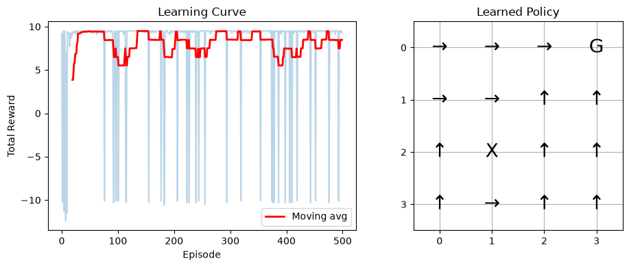
The agent learned to navigate to the goal (G) while avoiding the pit (X)!
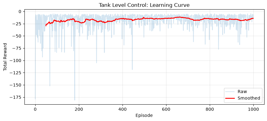
Example 2: Tank Level Control#
Now let’s apply RL to a real engineering problem: controlling the liquid level in a tank.
The System#
     Inlet (u)
        ↓
    ┌───────┐
    │       │ ← Level (h)
    │~~~~~~~│
    │       │
    └───┬───┘
        ↓
     Outlet (proportional to √h)
Dynamics: \(\frac{dh}{dt} = \frac{1}{A}(F_{in} - k\sqrt{h})\)
Where:
\(h\) = liquid level (our state)
\(F_{in}\) = inlet flow rate (our action)
\(A\) = tank cross-sectional area
\(k\) = outlet coefficient
Goal: Keep the level at a setpoint (e.g., h = 5.0)
class TankLevelEnv:
    """
    Tank level control environment.

    State: discretized level (0-10, in 20 bins)
    Actions: inlet flow rate (low, medium, high)
    Reward: negative squared error from setpoint
    """

    def __init__(self, setpoint=5.0, dt=0.5, max_steps=100):
        # Tank parameters
        self.A = 1.0      # Cross-sectional area
        self.k = 0.5      # Outlet coefficient

        # Control parameters
        self.setpoint = setpoint
        self.dt = dt
        self.max_steps = max_steps

        # State discretization (20 bins from 0 to 10)
        self.n_states = 20
        self.level_min = 0.0
        self.level_max = 10.0

        # Action space: 5 discrete flow rates
        self.flow_rates = [0.0, 0.5, 1.0, 1.5, 2.0]

        self.reset()

    def reset(self):
        """Reset to random initial level."""
        self.level = np.random.uniform(1.0, 9.0)
        self.steps = 0
        return self._discretize_state(self.level)

    def _discretize_state(self, level):
        """Convert continuous level to discrete state."""
        level = np.clip(level, self.level_min, self.level_max)
        bin_idx = int((level - self.level_min) / (self.level_max - self.level_min) * (self.n_states - 1))
        return min(bin_idx, self.n_states - 1)

    def step(self, action):
        """
        Take an action (set inlet flow rate).
        Returns: (state, reward, done)
        """
        F_in = self.flow_rates[action]

        # Simulate tank dynamics (Euler integration)
        F_out = self.k * np.sqrt(max(self.level, 0))
        dh_dt = (F_in - F_out) / self.A
        self.level = max(0, self.level + dh_dt * self.dt)

        # Calculate reward (negative squared error)
        error = self.level - self.setpoint
        reward = -error**2

        # Add small penalty for large flow changes (smooth control)
        reward -= 0.01 * F_in**2

        self.steps += 1
        done = self.steps >= self.max_steps

        return self._discretize_state(self.level), reward, done

    def get_actions(self):
        return list(range(len(self.flow_rates)))

    def get_continuous_level(self):
        """Get the actual continuous level (for plotting)."""
        return self.level
# Train Q-learning agent on tank control
tank_env = TankLevelEnv(setpoint=5.0)

# Train with decaying exploration
Q_tank, rewards_tank = q_learning(
    tank_env,
    n_episodes=1000,
    alpha=0.2,
    gamma=0.95,
    epsilon=0.2
)

# Plot learning curve
plt.figure(figsize=(10, 4))
window = 50
smoothed = np.convolve(rewards_tank, np.ones(window)/window, mode='valid')
plt.plot(rewards_tank, alpha=0.2, label='Raw')
plt.plot(range(window-1, len(rewards_tank)), smoothed, 'r-', linewidth=2, label='Smoothed')
plt.xlabel('Episode')
plt.ylabel('Total Reward')
plt.title('Tank Level Control: Learning Curve')
plt.legend()
plt.grid(True, alpha=0.3)
plt.show()
def run_episode_and_record(env, Q, epsilon=0.0):
    """Run one episode and record the trajectory."""
    state = env.reset()
    levels = [env.get_continuous_level()]
    actions_taken = []

    done = False
    while not done:
        if random.random() < epsilon:
            action = random.choice(env.get_actions())
        else:
            q_values = [Q[(state, a)] for a in env.get_actions()]
            action = np.argmax(q_values)

        state, reward, done = env.step(action)
        levels.append(env.get_continuous_level())
        actions_taken.append(env.flow_rates[action])

    return np.array(levels), np.array(actions_taken)

# Test the trained agent
tank_env_test = TankLevelEnv(setpoint=5.0)
levels, actions = run_episode_and_record(tank_env_test, Q_tank)

# Plot results
fig, axes = plt.subplots(2, 1, figsize=(10, 6), sharex=True)

time = np.arange(len(levels)) * tank_env_test.dt

axes[0].plot(time, levels, 'b-', linewidth=2, label='Level')
axes[0].axhline(y=5.0, color='r', linestyle='--', linewidth=2, label='Setpoint')
axes[0].set_ylabel('Tank Level')
axes[0].set_title('RL-Controlled Tank Level')
axes[0].legend()
axes[0].grid(True, alpha=0.3)

axes[1].step(time[:-1], actions, 'g-', linewidth=2, where='post')
axes[1].set_xlabel('Time')
axes[1].set_ylabel('Inlet Flow Rate')
axes[1].set_title('Control Action')
axes[1].grid(True, alpha=0.3)

plt.tight_layout()
plt.show()

print(f"Final level: {levels[-1]:.2f} (setpoint: 5.0)")
print(f"Mean squared error: {np.mean((levels - 5.0)**2):.4f}")
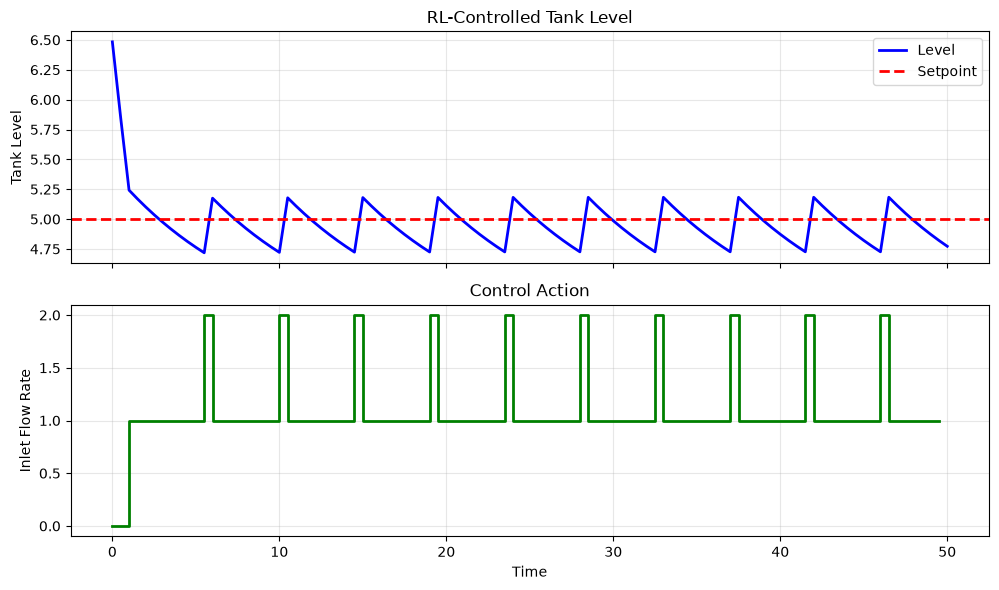
Final level: 4.77 (setpoint: 5.0)
Mean squared error: 0.0538
Comparison: RL vs PID Control#
Let’s compare our RL controller to a classical PID controller on the same problem.
class PIDController:
    """Simple PID controller."""

    def __init__(self, Kp, Ki, Kd, setpoint, dt):
        self.Kp = Kp
        self.Ki = Ki
        self.Kd = Kd
        self.setpoint = setpoint
        self.dt = dt
        self.integral = 0
        self.prev_error = 0

    def compute(self, measurement):
        error = self.setpoint - measurement

        # PID terms
        P = self.Kp * error
        self.integral += error * self.dt
        I = self.Ki * self.integral
        D = self.Kd * (error - self.prev_error) / self.dt

        self.prev_error = error

        # Output (clipped to valid flow rates)
        output = P + I + D
        return np.clip(output, 0, 2.0)

    def reset(self):
        self.integral = 0
        self.prev_error = 0


def run_pid_control(initial_level, setpoint, n_steps, dt):
    """Run tank simulation with PID control."""
    # Tank parameters
    A = 1.0
    k = 0.5

    # PID controller (manually tuned)
    pid = PIDController(Kp=0.8, Ki=0.1, Kd=0.2, setpoint=setpoint, dt=dt)

    level = initial_level
    levels = [level]
    actions = []

    for _ in range(n_steps):
        F_in = pid.compute(level)
        actions.append(F_in)

        # Simulate
        F_out = k * np.sqrt(max(level, 0))
        dh_dt = (F_in - F_out) / A
        level = max(0, level + dh_dt * dt)
        levels.append(level)

    return np.array(levels), np.array(actions)
# Run both controllers from the same initial condition
initial_level = 2.0
setpoint = 5.0
n_steps = 100
dt = 0.5

# PID control
levels_pid, actions_pid = run_pid_control(initial_level, setpoint, n_steps, dt)

# RL control (set initial condition manually)
tank_env_compare = TankLevelEnv(setpoint=setpoint)
tank_env_compare.reset()
tank_env_compare.level = initial_level
levels_rl, actions_rl = run_episode_and_record(tank_env_compare, Q_tank)

# Plot comparison
fig, axes = plt.subplots(2, 1, figsize=(12, 7), sharex=True)

time_pid = np.arange(len(levels_pid)) * dt
time_rl = np.arange(len(levels_rl)) * dt

# Level comparison
axes[0].plot(time_pid, levels_pid, 'b-', linewidth=2, label='PID')
axes[0].plot(time_rl, levels_rl, 'g-', linewidth=2, label='RL (Q-learning)')
axes[0].axhline(y=setpoint, color='r', linestyle='--', linewidth=2, label='Setpoint')
axes[0].set_ylabel('Tank Level')
axes[0].set_title('PID vs RL Control Comparison')
axes[0].legend()
axes[0].grid(True, alpha=0.3)

# Action comparison
axes[1].plot(time_pid[:-1], actions_pid, 'b-', linewidth=2, label='PID')
axes[1].step(time_rl[:-1], actions_rl, 'g-', linewidth=2, where='post', label='RL')
axes[1].set_xlabel('Time')
axes[1].set_ylabel('Inlet Flow Rate')
axes[1].legend()
axes[1].grid(True, alpha=0.3)

plt.tight_layout()
plt.show()

# Performance metrics
mse_pid = np.mean((levels_pid - setpoint)**2)
mse_rl = np.mean((levels_rl - setpoint)**2)

print(f"\nPerformance Comparison:")
print(f"  PID Mean Squared Error: {mse_pid:.4f}")
print(f"  RL  Mean Squared Error: {mse_rl:.4f}")
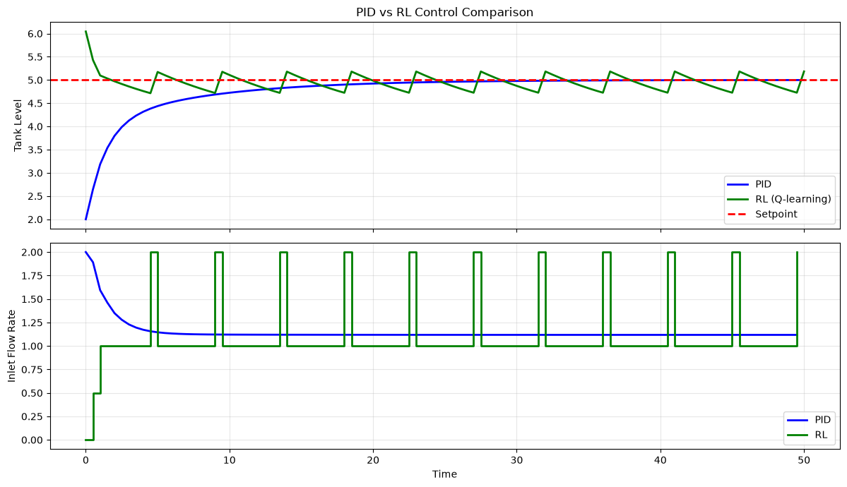
Performance Comparison:
  PID Mean Squared Error: 0.2677
  RL  Mean Squared Error: 0.0378
Observations:
PID provides smooth, continuous control with well-understood behavior
RL learns discrete actions that may be less smooth but can handle complex scenarios
For simple setpoint tracking, PID often works well
RL shines when dynamics are complex, nonlinear, or hard to model
Example 3: Battery Energy Management#
Now let’s tackle a resource management problem: optimizing battery charging and discharging to minimize electricity costs given time-varying prices.
Scenario:
Battery with limited capacity
Electricity prices vary throughout the day (cheap at night, expensive during peak)
Goal: Buy low, sell high (or use stored energy during peak)
This is harder than the tank problem because the optimal action depends on future prices, not just current state.
class BatteryEnv:
    """
    Battery energy management environment.

    State: (hour_of_day, battery_level)
    Actions: charge, hold, discharge
    Reward: negative cost (minimize buying at high prices)
    """

    def __init__(self, capacity=10.0, charge_rate=2.0, efficiency=0.9):
        self.capacity = capacity
        self.charge_rate = charge_rate
        self.efficiency = efficiency

        # Discretize battery level into 10 bins
        self.n_battery_states = 11  # 0%, 10%, ..., 100%

        # 24 hours in a day
        self.n_hours = 24

        # Price profile (simplified): cheap at night, expensive afternoon
        self.prices = self._generate_price_profile()

        # Base load (energy needed regardless of battery)
        self.base_load = 1.0

        self.reset()

    def _generate_price_profile(self):
        """Generate realistic daily price profile."""
        hours = np.arange(24)
        # Low at night (0-6), rising morning, peak afternoon (14-18), declining evening
        prices = 0.05 + 0.10 * np.exp(-((hours - 16)**2) / 20) + 0.03 * np.sin(hours * np.pi / 12)
        return prices

    def reset(self):
        """Reset to start of day with random battery level."""
        self.hour = 0
        self.battery = np.random.uniform(0.2, 0.8) * self.capacity
        return self._get_state()

    def _get_state(self):
        """Return discretized state (hour, battery_level_bin)."""
        battery_bin = int(self.battery / self.capacity * (self.n_battery_states - 1))
        battery_bin = np.clip(battery_bin, 0, self.n_battery_states - 1)
        return (self.hour, battery_bin)

    def step(self, action):
        """
        Take action: 0=charge, 1=hold, 2=discharge
        """
        price = self.prices[self.hour]

        # Calculate energy flows
        if action == 0:  # Charge
            energy_bought = self.charge_rate
            energy_stored = energy_bought * self.efficiency
            self.battery = min(self.capacity, self.battery + energy_stored)
            grid_energy = self.base_load + energy_bought
        elif action == 1:  # Hold
            grid_energy = self.base_load
        else:  # Discharge
            energy_available = min(self.battery, self.charge_rate)
            self.battery -= energy_available
            # Use battery energy to offset base load
            grid_energy = max(0, self.base_load - energy_available * self.efficiency)

        # Cost = price * energy from grid
        cost = price * grid_energy
        reward = -cost  # Minimize cost

        self.hour += 1
        done = self.hour >= self.n_hours

        return self._get_state(), reward, done

    def get_actions(self):
        return [0, 1, 2]  # charge, hold, discharge

    def get_battery_level(self):
        return self.battery

    def get_price(self, hour):
        return self.prices[hour]
# Visualize the price profile
battery_env = BatteryEnv()
hours = np.arange(24)

plt.figure(figsize=(10, 4))
plt.bar(hours, battery_env.prices, color='steelblue', alpha=0.7)
plt.xlabel('Hour of Day')
plt.ylabel('Electricity Price ($/kWh)')
plt.title('Daily Electricity Price Profile')
plt.xticks(hours)
plt.grid(True, alpha=0.3, axis='y')
plt.show()

print("Cheap hours: 0-6 (night), Expensive hours: 14-18 (afternoon peak)")
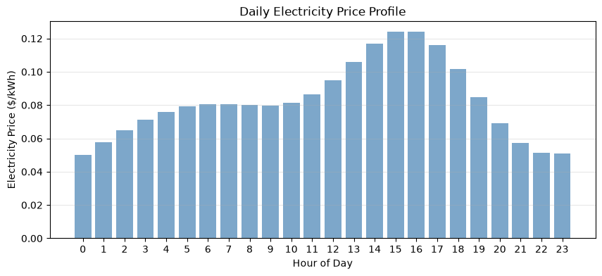
Cheap hours: 0-6 (night), Expensive hours: 14-18 (afternoon peak)
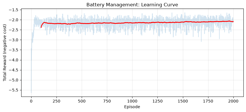
# Train RL agent on battery management
battery_env = BatteryEnv()

Q_battery, rewards_battery = q_learning(
    battery_env,
    n_episodes=2000,
    alpha=0.1,
    gamma=0.99,
    epsilon=0.15
)

# Plot learning curve
plt.figure(figsize=(10, 4))
window = 100
smoothed = np.convolve(rewards_battery, np.ones(window)/window, mode='valid')
plt.plot(rewards_battery, alpha=0.2)
plt.plot(range(window-1, len(rewards_battery)), smoothed, 'r-', linewidth=2)
plt.xlabel('Episode')
plt.ylabel('Total Reward (negative cost)')
plt.title('Battery Management: Learning Curve')
plt.grid(True, alpha=0.3)
plt.show()
def run_battery_episode(env, Q, epsilon=0.0):
    """Run one day and record everything."""
    state = env.reset()

    hours = [0]
    battery_levels = [env.get_battery_level()]
    actions = []
    costs = []
    prices = [env.get_price(0)]

    done = False
    while not done:
        if random.random() < epsilon:
            action = random.choice(env.get_actions())
        else:
            q_values = [Q[(state, a)] for a in env.get_actions()]
            action = np.argmax(q_values)

        state, reward, done = env.step(action)

        hours.append(env.hour)
        battery_levels.append(env.get_battery_level())
        actions.append(action)
        costs.append(-reward)
        if not done:
            prices.append(env.get_price(env.hour))

    return hours, battery_levels, actions, costs, prices

# Test the trained agent
battery_test = BatteryEnv()
hours, battery_levels, actions, costs, prices = run_battery_episode(battery_test, Q_battery)

# Plot results
fig, axes = plt.subplots(3, 1, figsize=(12, 9), sharex=True)

# Price profile
axes[0].bar(hours[:-1], prices, color='steelblue', alpha=0.7)
axes[0].set_ylabel('Price ($/kWh)')
axes[0].set_title('Electricity Price')
axes[0].grid(True, alpha=0.3, axis='y')

# Battery level
axes[1].plot(hours, battery_levels, 'g-', linewidth=2, marker='o', markersize=4)
axes[1].axhline(y=battery_test.capacity, color='r', linestyle='--', alpha=0.5, label='Max capacity')
axes[1].set_ylabel('Battery Level (kWh)')
axes[1].set_title('Battery State of Charge')
axes[1].legend()
axes[1].grid(True, alpha=0.3)

# Actions taken
action_names = ['Charge', 'Hold', 'Discharge']
action_colors = ['green', 'gray', 'red']
for i, (h, a) in enumerate(zip(hours[:-1], actions)):
    axes[2].bar(h, 1, color=action_colors[a], alpha=0.7)
axes[2].set_xlabel('Hour of Day')
axes[2].set_ylabel('Action')
axes[2].set_yticks([0.5])
axes[2].set_yticklabels([''])
axes[2].set_title('Actions: Green=Charge, Gray=Hold, Red=Discharge')

plt.tight_layout()
plt.show()

total_cost = sum(costs)
print(f"\nTotal daily cost: ${total_cost:.2f}")
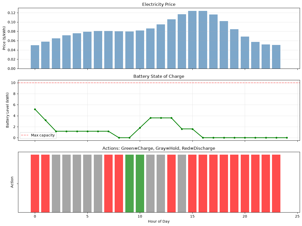
Total daily cost: $1.89
# Compare to naive strategy (always hold)
def naive_battery_strategy(env):
    """Baseline: never use the battery."""
    env.reset()
    total_cost = 0
    done = False
    while not done:
        _, reward, done = env.step(1)  # Always hold
        total_cost -= reward
    return total_cost

def simple_rule_strategy(env):
    """Simple rule: charge when cheap (<0.06), discharge when expensive (>0.10)."""
    env.reset()
    total_cost = 0
    done = False
    hour = 0
    while not done:
        price = env.get_price(hour)
        if price < 0.06:
            action = 0  # Charge
        elif price > 0.10:
            action = 2  # Discharge
        else:
            action = 1  # Hold
        _, reward, done = env.step(action)
        total_cost -= reward
        hour += 1
    return total_cost

# Run comparison
n_trials = 100
rl_costs = []
naive_costs = []
rule_costs = []

for _ in range(n_trials):
    # RL agent
    env = BatteryEnv()
    _, _, _, costs, _ = run_battery_episode(env, Q_battery)
    rl_costs.append(sum(costs))

    # Naive
    env = BatteryEnv()
    naive_costs.append(naive_battery_strategy(env))

    # Rule-based
    env = BatteryEnv()
    rule_costs.append(simple_rule_strategy(env))

print("Average Daily Cost Comparison (100 trials):")
print(f"  Naive (no battery use): ${np.mean(naive_costs):.2f} ± ${np.std(naive_costs):.2f}")
print(f"  Simple Rule-based:      ${np.mean(rule_costs):.2f} ± ${np.std(rule_costs):.2f}")
print(f"  RL (Q-learning):        ${np.mean(rl_costs):.2f} ± ${np.std(rl_costs):.2f}")
print(f"\nRL saves ${np.mean(naive_costs) - np.mean(rl_costs):.2f}/day vs naive")
Average Daily Cost Comparison (100 trials):
  Naive (no battery use): $1.99 ± $0.00
  Simple Rule-based:      $2.01 ± $0.08
  RL (Q-learning):        $1.95 ± $0.10

RL saves $0.04/day vs naive
Using Libraries: Gymnasium and Stable-Baselines3#
For more complex problems, we use established libraries:
Gymnasium: Standard API for RL environments
Stable-Baselines3: Production-quality RL algorithms (DQN, PPO, A2C, etc.)
Let’s wrap our tank control problem as a proper Gymnasium environment.
# Check if gymnasium and stable-baselines3 are available
try:
    import gymnasium as gym
    from gymnasium import spaces
    GYM_AVAILABLE = True
    print("Gymnasium is available!")
except ImportError:
    GYM_AVAILABLE = False
    print("Gymnasium not installed. Install with: pip install gymnasium")

try:
    from stable_baselines3 import PPO, DQN
    from stable_baselines3.common.evaluation import evaluate_policy
    SB3_AVAILABLE = True
    print("Stable-Baselines3 is available!")
except ImportError:
    SB3_AVAILABLE = False
    print("Stable-Baselines3 not installed. Install with: pip install stable-baselines3")
Gymnasium not installed. Install with: pip install gymnasium
Stable-Baselines3 not installed. Install with: pip install stable-baselines3
if GYM_AVAILABLE:
    class TankLevelGymEnv(gym.Env):
        """
        Tank level control as a Gymnasium environment.

        This uses continuous state and action spaces,
        suitable for deep RL algorithms like PPO.
        """

        metadata = {'render_modes': ['human']}

        def __init__(self, setpoint=5.0, dt=0.5, max_steps=100):
            super().__init__()

            # Tank parameters
            self.A = 1.0
            self.k = 0.5
            self.setpoint = setpoint
            self.dt = dt
            self.max_steps = max_steps

            # Continuous action space: flow rate from 0 to 2
            self.action_space = spaces.Box(
                low=0.0, high=2.0, shape=(1,), dtype=np.float32
            )

            # Continuous observation: [level, error, setpoint]
            self.observation_space = spaces.Box(
                low=np.array([0.0, -10.0, 0.0]),
                high=np.array([10.0, 10.0, 10.0]),
                dtype=np.float32
            )

            self.level = 5.0
            self.steps = 0

        def reset(self, seed=None, options=None):
            super().reset(seed=seed)
            self.level = self.np_random.uniform(1.0, 9.0)
            self.steps = 0
            return self._get_obs(), {}

        def _get_obs(self):
            error = self.level - self.setpoint
            return np.array([self.level, error, self.setpoint], dtype=np.float32)

        def step(self, action):
            F_in = float(action[0])
            F_in = np.clip(F_in, 0.0, 2.0)

            # Simulate tank dynamics
            F_out = self.k * np.sqrt(max(self.level, 0))
            dh_dt = (F_in - F_out) / self.A
            self.level = max(0, min(10, self.level + dh_dt * self.dt))

            # Reward: negative squared error + small control penalty
            error = self.level - self.setpoint
            reward = -error**2 - 0.01 * F_in**2

            self.steps += 1
            terminated = False
            truncated = self.steps >= self.max_steps

            return self._get_obs(), reward, terminated, truncated, {}

    print("TankLevelGymEnv class defined!")
else:
    print("Skipping Gymnasium environment definition.")
Skipping Gymnasium environment definition.
if GYM_AVAILABLE and SB3_AVAILABLE:
    # Create environment
    env = TankLevelGymEnv(setpoint=5.0)

    # Train PPO agent
    print("Training PPO agent (this may take a minute)...")
    model = PPO(
        "MlpPolicy",
        env,
        verbose=0,
        learning_rate=3e-4,
        n_steps=1024,
        batch_size=64,
        n_epochs=10,
        gamma=0.99
    )
    model.learn(total_timesteps=50000)
    print("Training complete!")

    # Evaluate
    mean_reward, std_reward = evaluate_policy(model, env, n_eval_episodes=10)
    print(f"Mean reward: {mean_reward:.2f} +/- {std_reward:.2f}")
else:
    print("Skipping PPO training (gymnasium or stable-baselines3 not available).")
Skipping PPO training (gymnasium or stable-baselines3 not available).
if GYM_AVAILABLE and SB3_AVAILABLE:
    # Test the trained PPO agent
    env = TankLevelGymEnv(setpoint=5.0)
    obs, _ = env.reset()

    levels = [obs[0]]
    actions_ppo = []

    for _ in range(100):
        action, _ = model.predict(obs, deterministic=True)
        obs, reward, terminated, truncated, _ = env.step(action)
        levels.append(obs[0])
        actions_ppo.append(action[0])
        if terminated or truncated:
            break

    # Plot PPO results
    fig, axes = plt.subplots(2, 1, figsize=(10, 6), sharex=True)

    time = np.arange(len(levels)) * 0.5

    axes[0].plot(time, levels, 'b-', linewidth=2)
    axes[0].axhline(y=5.0, color='r', linestyle='--', linewidth=2, label='Setpoint')
    axes[0].set_ylabel('Tank Level')
    axes[0].set_title('PPO-Controlled Tank Level (Deep RL)')
    axes[0].legend()
    axes[0].grid(True, alpha=0.3)

    axes[1].plot(time[:-1], actions_ppo, 'g-', linewidth=2)
    axes[1].set_xlabel('Time')
    axes[1].set_ylabel('Inlet Flow Rate')
    axes[1].set_title('Control Action (Continuous)')
    axes[1].grid(True, alpha=0.3)

    plt.tight_layout()
    plt.show()

    print(f"Final level: {levels[-1]:.2f}")
    print(f"MSE: {np.mean((np.array(levels) - 5.0)**2):.4f}")
else:
    print("Skipping PPO test visualization.")
Skipping PPO test visualization.
Practical Tips for RL in Engineering#
1. Reward Shaping is Critical#
The reward function is how you communicate goals to the agent. Common patterns:
Goal |
Reward Design |
|---|---|
Setpoint tracking |
|
Smooth control |
Add penalty: |
Safety constraints |
Large negative reward for violations |
Efficiency |
|
2. State Representation Matters#
Include information the agent needs to make good decisions:
Current measurement
Error from setpoint
Rate of change (derivative)
Time or phase information (for cyclic processes)
3. Start Simple, Then Scale#
Start with tabular Q-learning on a discretized problem
Verify it learns reasonable behavior
Move to deep RL (PPO, SAC) for continuous/complex problems
4. Simulation Fidelity#
Train in simulation, deploy on real system
The simulation must capture important dynamics
Add noise during training for robustness
5. When to Use RL vs Classical Control#
Use Classical (PID, MPC) |
Use RL |
|---|---|
Well-understood dynamics |
Complex, nonlinear dynamics |
Single objective |
Multiple competing objectives |
Safety-critical |
Simulation is cheap |
Need interpretability |
Can learn from data |
Fast tuning possible |
Long-horizon planning needed |
Summary#
This chapter introduced Reinforcement Learning for engineering applications:
The RL Framework: Agent, environment, state, action, reward. The agent learns a policy to maximize cumulative reward.
Q-Learning from Scratch: Built a simple tabular Q-learning algorithm. Key concepts:
Q-values estimate future reward
ε-greedy balances exploration and exploitation
Learning rate and discount factor control updates
Control Problem: Tank level control
Discretized state and action spaces
Compared RL to PID control
Both work; RL learns from experience, PID from tuning
Resource Management: Battery optimization
Time-varying prices require planning ahead
RL learned to charge when cheap, discharge when expensive
Outperformed simple rule-based strategies
Libraries: Gymnasium + Stable-Baselines3
Standard API for environments
PPO for continuous control
Production-ready implementations
Key Takeaway: RL is powerful for sequential decision-making when you can simulate the system. Start simple (tabular Q-learning), verify behavior, then scale to deep RL for complex problems.