
Parallel Processing in Python#
KEYWORDS: multiprocessing, threading, concurrent.futures, joblib, parallel computing
Introduction#
Many computational tasks in science and engineering are embarrassingly parallel - they can be broken into independent pieces that run simultaneously. Examples include:
Parameter sweeps: solving an ODE with 1000 different rate constants
Monte Carlo simulations: running 10,000 random trials for uncertainty quantification
Batch processing: analyzing hundreds of experimental data files
Cross-validation: training models on different data subsets
Modern computers have multiple CPU cores, but Python code runs on a single core by default. This chapter shows you how to use all your cores effectively.
import numpy as np
import matplotlib.pyplot as plt
import time
import os

# How many CPU cores do we have?
print(f"Available CPU cores: {os.cpu_count()}")
Available CPU cores: 4
CPU-bound vs I/O-bound Tasks#
Before diving into parallel processing, we need to understand two types of tasks:
CPU-bound tasks spend most of their time doing computation:
Numerical integration
Matrix operations
Solving differential equations
Image processing algorithms
I/O-bound tasks spend most of their time waiting for input/output:
Reading/writing files
Network requests (downloading data, API calls)
Database queries
This distinction is critical because Python’s Global Interpreter Lock (GIL) affects how we parallelize each type.
The Global Interpreter Lock (GIL)#
Python has a mechanism called the Global Interpreter Lock (GIL) that allows only one thread to execute Python bytecode at a time. This was a design decision to simplify memory management in CPython.
Implications:
Threads do NOT speed up CPU-bound Python code (they actually run one at a time!)
Threads DO speed up I/O-bound code (while one thread waits for I/O, another can run)
Processes bypass the GIL entirely (each process has its own Python interpreter)
This is why we use:
threadingfor I/O-bound tasks (file operations, network requests)multiprocessingfor CPU-bound tasks (numerical computations)
Let’s demonstrate this with a simple example.
def cpu_intensive_task(n):
    """A CPU-bound task: compute sum of squares."""
    total = 0
    for i in range(n):
        total += i ** 2
    return total

# Time a single call
n = 1_000_000
start = time.perf_counter()
result = cpu_intensive_task(n)
elapsed = time.perf_counter() - start
print(f"Single call: {elapsed:.3f} seconds")
Single call: 0.061 seconds
Threading: For I/O-bound Tasks#
The threading module creates lightweight threads that share memory. They’re ideal for I/O-bound tasks where threads spend time waiting.
Example: Simulating I/O with sleep#
Let’s simulate reading multiple data files (using time.sleep to represent I/O wait time).
import threading

def simulate_file_read(file_id, results):
    """Simulate reading a file (I/O-bound task)."""
    time.sleep(0.5)  # Simulate I/O wait
    results[file_id] = f"Data from file {file_id}"

# Sequential approach
n_files = 5
results_seq = {}

start = time.perf_counter()
for i in range(n_files):
    simulate_file_read(i, results_seq)
sequential_time = time.perf_counter() - start
print(f"Sequential: {sequential_time:.2f} seconds")

# Threaded approach
results_threaded = {}
threads = []

start = time.perf_counter()
for i in range(n_files):
    t = threading.Thread(target=simulate_file_read, args=(i, results_threaded))
    threads.append(t)
    t.start()

# Wait for all threads to complete
for t in threads:
    t.join()

threaded_time = time.perf_counter() - start
print(f"Threaded: {threaded_time:.2f} seconds")
print(f"Speedup: {sequential_time / threaded_time:.1f}x")
Sequential: 2.50 seconds
Threaded: 0.50 seconds
Speedup: 5.0x
The threaded version is ~5x faster because all threads can wait for I/O simultaneously.
Why threads DON’T help with CPU-bound tasks#
Let’s try the same approach with our CPU-intensive function:
def cpu_task_wrapper(n, results, idx):
    results[idx] = cpu_intensive_task(n)

n = 500_000
n_tasks = 4

# Sequential
results_seq = {}
start = time.perf_counter()
for i in range(n_tasks):
    results_seq[i] = cpu_intensive_task(n)
sequential_time = time.perf_counter() - start
print(f"Sequential: {sequential_time:.3f} seconds")

# Threaded (won't help due to GIL!)
results_threaded = {}
threads = []

start = time.perf_counter()
for i in range(n_tasks):
    t = threading.Thread(target=cpu_task_wrapper, args=(n, results_threaded, i))
    threads.append(t)
    t.start()

for t in threads:
    t.join()

threaded_time = time.perf_counter() - start
print(f"Threaded: {threaded_time:.3f} seconds")
print(f"Speedup: {sequential_time / threaded_time:.2f}x (no improvement due to GIL!)")
Sequential: 0.118 seconds
Threaded: 0.133 seconds
Speedup: 0.89x (no improvement due to GIL!)
Notice that threading provides no speedup (and may even be slower due to overhead). The GIL ensures only one thread runs Python code at a time.
Multiprocessing: For CPU-bound Tasks#
The multiprocessing module creates separate Python processes, each with its own GIL. This allows true parallel execution on multiple cores.
Example: Parameter Sweep for Reaction Kinetics#
Consider a first-order reaction \(A \rightarrow B\) with rate \(r = k C_A\). We want to study how the final conversion depends on the rate constant \(k\). This requires solving the ODE:
for many different values of \(k\).
from scipy.integrate import solve_ivp

def solve_reaction(k, C_A0=1.0, t_final=10.0):
    """Solve first-order reaction kinetics for a given rate constant k.

    Returns the final conversion X = (C_A0 - C_A) / C_A0
    """
    def ode(t, C):
        C_A = C[0]
        return [-k * C_A]

    sol = solve_ivp(ode, [0, t_final], [C_A0], dense_output=True)
    C_A_final = sol.y[0, -1]
    conversion = (C_A0 - C_A_final) / C_A0
    return k, conversion

# Test it
k_test, conv_test = solve_reaction(0.5)
print(f"k = {k_test}, conversion = {conv_test:.4f}")
k = 0.5, conversion = 0.9932
import multiprocessing as mp

# Generate 200 rate constants to test
k_values = np.linspace(0.01, 2.0, 200)

# Sequential approach
start = time.perf_counter()
results_seq = [solve_reaction(k) for k in k_values]
sequential_time = time.perf_counter() - start
print(f"Sequential: {sequential_time:.3f} seconds")

# Parallel approach using multiprocessing Pool
start = time.perf_counter()
with mp.Pool(processes=mp.cpu_count()) as pool:
    results_parallel = pool.map(solve_reaction, k_values)
parallel_time = time.perf_counter() - start
print(f"Parallel ({mp.cpu_count()} cores): {parallel_time:.3f} seconds")
print(f"Speedup: {sequential_time / parallel_time:.2f}x")
Sequential: 0.120 seconds
Parallel (4 cores): 0.127 seconds
Speedup: 0.94x
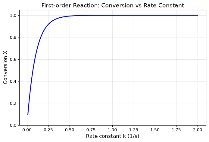
# Visualize the results
k_vals = [r[0] for r in results_parallel]
conversions = [r[1] for r in results_parallel]

plt.figure(figsize=(8, 5))
plt.plot(k_vals, conversions, 'b-', linewidth=2)
plt.xlabel('Rate constant k (1/s)', fontsize=12)
plt.ylabel('Conversion X', fontsize=12)
plt.title('First-order Reaction: Conversion vs Rate Constant', fontsize=14)
plt.grid(True, alpha=0.3)
plt.ylim(0, 1.05);
Important Notes about Multiprocessing#
Pickling: Data passed between processes must be picklable (serializable). Most numpy arrays and simple objects work fine, but lambda functions and some objects don’t.
Overhead: Creating processes has overhead. For very fast tasks, the overhead may exceed the benefit.
Memory: Each process has its own memory space. Large data is copied to each process.
Top-level functions: Functions used with
Pool.map()must be defined at the module level (not inside another function).
concurrent.futures: The Modern Interface#
The concurrent.futures module provides a clean, unified API for both threading and multiprocessing. It’s the recommended approach for most parallel tasks.
ThreadPoolExecutor: For I/O-bound tasksProcessPoolExecutor: For CPU-bound tasks
Both have the same interface, making it easy to switch between them.
from concurrent.futures import ProcessPoolExecutor, ThreadPoolExecutor, as_completed

# Using ProcessPoolExecutor for our reaction kinetics
start = time.perf_counter()
with ProcessPoolExecutor(max_workers=mp.cpu_count()) as executor:
    # map() returns results in order
    results = list(executor.map(solve_reaction, k_values))
elapsed = time.perf_counter() - start
print(f"ProcessPoolExecutor: {elapsed:.3f} seconds")
ProcessPoolExecutor: 0.147 seconds
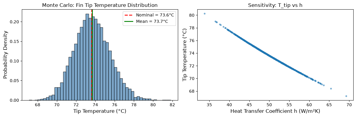
Example: Monte Carlo Uncertainty Quantification#
A powerful application of parallel processing is Monte Carlo simulation. Suppose we’re measuring the heat transfer coefficient \(h\) for a cooling fin, and we want to estimate the uncertainty in the steady-state temperature.
The fin equation gives us: $\(T(x) = T_\infty + (T_0 - T_\infty) \frac{\cosh(m(L-x))}{\cosh(mL)}\)$
where \(m = \sqrt{\frac{hP}{kA}}\).
If \(h\) has measurement uncertainty (normally distributed), what’s the distribution of the tip temperature \(T(L)\)?
def fin_tip_temperature(h, T0=100, T_inf=25, L=0.1, k=200, P=0.04, A=1e-4):
    """
    Calculate the tip temperature of a cooling fin.

    Parameters:
    -----------
    h : float
        Heat transfer coefficient (W/m^2-K)
    T0 : float
        Base temperature (°C)
    T_inf : float
        Ambient temperature (°C)
    L : float
        Fin length (m)
    k : float
        Thermal conductivity (W/m-K)
    P : float
        Perimeter (m)
    A : float
        Cross-sectional area (m^2)
    """
    m = np.sqrt(h * P / (k * A))
    T_tip = T_inf + (T0 - T_inf) / np.cosh(m * L)
    return T_tip

# Nominal value
h_nominal = 50  # W/m^2-K
T_nominal = fin_tip_temperature(h_nominal)
print(f"Nominal tip temperature: {T_nominal:.2f} °C")
Nominal tip temperature: 73.60 °C
# Monte Carlo simulation with uncertainty in h
np.random.seed(42)
n_samples = 10000
h_std = 5  # Standard deviation in h measurement

# Generate random samples of h
h_samples = np.random.normal(h_nominal, h_std, n_samples)
h_samples = h_samples[h_samples > 0]  # h must be positive

# Sequential Monte Carlo
start = time.perf_counter()
T_results_seq = [fin_tip_temperature(h) for h in h_samples]
sequential_time = time.perf_counter() - start
print(f"Sequential: {sequential_time:.3f} seconds")

# Parallel Monte Carlo
start = time.perf_counter()
with ProcessPoolExecutor() as executor:
    T_results_parallel = list(executor.map(fin_tip_temperature, h_samples))
parallel_time = time.perf_counter() - start
print(f"Parallel: {parallel_time:.3f} seconds")
Sequential: 0.008 seconds
Parallel: 2.375 seconds
# Analyze and visualize results
T_array = np.array(T_results_parallel)

fig, axes = plt.subplots(1, 2, figsize=(12, 4))

# Histogram of tip temperatures
axes[0].hist(T_array, bins=50, density=True, alpha=0.7, color='steelblue', edgecolor='black')
axes[0].axvline(T_nominal, color='red', linestyle='--', linewidth=2, label=f'Nominal = {T_nominal:.1f}°C')
axes[0].axvline(T_array.mean(), color='green', linestyle='-', linewidth=2, label=f'Mean = {T_array.mean():.1f}°C')
axes[0].set_xlabel('Tip Temperature (°C)', fontsize=12)
axes[0].set_ylabel('Probability Density', fontsize=12)
axes[0].set_title('Monte Carlo: Fin Tip Temperature Distribution', fontsize=12)
axes[0].legend()

# Scatter plot: h vs T_tip
axes[1].scatter(h_samples[:1000], T_array[:1000], alpha=0.5, s=10)
axes[1].set_xlabel('Heat Transfer Coefficient h (W/m²K)', fontsize=12)
axes[1].set_ylabel('Tip Temperature (°C)', fontsize=12)
axes[1].set_title('Sensitivity: T_tip vs h', fontsize=12)

plt.tight_layout()

print(f"\nMonte Carlo Results ({len(T_array)} samples):")
print(f"  Mean tip temperature: {T_array.mean():.2f} °C")
print(f"  Standard deviation: {T_array.std():.2f} °C")
print(f"  95% confidence interval: [{np.percentile(T_array, 2.5):.2f}, {np.percentile(T_array, 97.5):.2f}] °C")
Monte Carlo Results (10000 samples):
  Mean tip temperature: 73.66 °C
  Standard deviation: 1.86 °C
  95% confidence interval: [70.16, 77.48] °C
Using submit() and as_completed()#
Sometimes you want to process results as they become available, rather than waiting for all tasks to complete. The submit() method returns Future objects, and as_completed() yields them as they finish.
def slow_computation(x):
    """A computation that takes variable time."""
    sleep_time = np.random.uniform(0.1, 0.5)
    time.sleep(sleep_time)
    return x ** 2, sleep_time

# Process results as they complete
values = list(range(8))

with ProcessPoolExecutor(max_workers=4) as executor:
    # Submit all tasks
    future_to_value = {executor.submit(slow_computation, v): v for v in values}

    # Process as they complete (not in submission order)
    for future in as_completed(future_to_value):
        original_value = future_to_value[future]
        result, elapsed = future.result()
        print(f"  {original_value}² = {result} (took {elapsed:.2f}s)")
  0² = 0 (took 0.23s)
  2² = 4 (took 0.23s)
  3² = 9 (took 0.23s)
  1² = 1 (took 0.23s)
  4² = 16 (took 0.14s)
  5² = 25 (took 0.14s)
  6² = 36 (took 0.14s)
  7² = 49 (took 0.14s)
Error Handling in Parallel Code#
When running many parallel tasks, some may fail. It’s important to handle errors gracefully.
def risky_computation(x):
    """A computation that might fail."""
    if x == 5:
        raise ValueError(f"Cannot process x={x}")
    return x ** 2

values = list(range(10))
results = []
errors = []

with ProcessPoolExecutor(max_workers=4) as executor:
    future_to_value = {executor.submit(risky_computation, v): v for v in values}

    for future in as_completed(future_to_value):
        value = future_to_value[future]
        try:
            result = future.result()
            results.append((value, result))
        except Exception as e:
            errors.append((value, str(e)))

print(f"Successful: {len(results)} tasks")
print(f"Failed: {len(errors)} tasks")
if errors:
    print(f"Errors: {errors}")
Successful: 9 tasks
Failed: 1 tasks
Errors: [(5, 'Cannot process x=5')]
Joblib: Parallel Computing Made Easy#
Joblib is a popular library in the scientific Python ecosystem. It’s used internally by scikit-learn and provides a simple interface for parallel computing.
Key features:
Simple
ParallelanddelayedsyntaxAutomatic backend selection (processes or threads)
Built-in progress reporting
Memory mapping for large numpy arrays
Result caching with
Memory
from joblib import Parallel, delayed

# Basic syntax: Parallel(n_jobs=...)(delayed(func)(args) for args in iterable)

# Sequential
start = time.perf_counter()
results_seq = [solve_reaction(k) for k in k_values]
print(f"Sequential: {time.perf_counter() - start:.3f}s")

# Parallel with joblib
start = time.perf_counter()
results_joblib = Parallel(n_jobs=-1)(  # n_jobs=-1 uses all cores
    delayed(solve_reaction)(k) for k in k_values
)
print(f"Joblib parallel: {time.perf_counter() - start:.3f}s")
Sequential: 0.120s
Joblib parallel: 1.183s
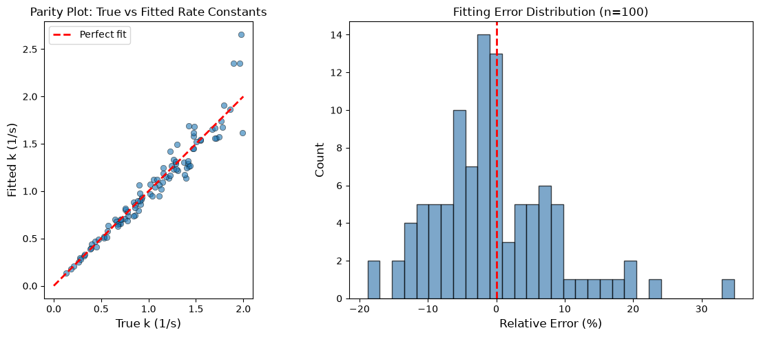
Example: Batch Processing Experimental Data#
Suppose we have experimental data from multiple runs of a reaction, and we want to fit a kinetic model to each dataset. This is a perfect use case for parallel processing.
from scipy.optimize import curve_fit

def first_order_model(t, k, C0):
    """First-order decay: C(t) = C0 * exp(-k*t)"""
    return C0 * np.exp(-k * t)

def generate_synthetic_data(true_k, true_C0, noise_level=0.05):
    """Generate synthetic experimental data with noise."""
    t = np.linspace(0, 10, 20)
    C_true = first_order_model(t, true_k, true_C0)
    C_noisy = C_true + np.random.normal(0, noise_level * true_C0, len(t))
    C_noisy = np.maximum(C_noisy, 0)  # Concentration can't be negative
    return t, C_noisy, true_k, true_C0

def fit_kinetic_model(data):
    """Fit first-order model to experimental data."""
    t, C, true_k, true_C0 = data
    try:
        popt, pcov = curve_fit(first_order_model, t, C, p0=[0.5, 1.0], bounds=(0, [10, 10]))
        k_fit, C0_fit = popt
        k_err = np.sqrt(pcov[0, 0])
        return {
            'true_k': true_k,
            'fitted_k': k_fit,
            'k_error': k_err,
            'true_C0': true_C0,
            'fitted_C0': C0_fit
        }
    except Exception as e:
        return {'error': str(e)}

# Generate 100 synthetic experiments with different true parameters
np.random.seed(123)
n_experiments = 100
true_k_values = np.random.uniform(0.1, 2.0, n_experiments)
true_C0_values = np.random.uniform(0.5, 2.0, n_experiments)

datasets = [
    generate_synthetic_data(k, C0)
    for k, C0 in zip(true_k_values, true_C0_values)
]
# Fit all experiments in parallel with progress reporting
start = time.perf_counter()
fit_results = Parallel(n_jobs=-1, verbose=1)(
    delayed(fit_kinetic_model)(data) for data in datasets
)
elapsed = time.perf_counter() - start
print(f"\nFitted {n_experiments} experiments in {elapsed:.2f} seconds")
Fitted 100 experiments in 0.15 seconds
[Parallel(n_jobs=-1)]: Using backend LokyBackend with 4 concurrent workers.
[Parallel(n_jobs=-1)]: Done 100 out of 100 | elapsed:    0.1s finished
# Analyze the fitting results
successful_fits = [r for r in fit_results if 'error' not in r]

true_k = np.array([r['true_k'] for r in successful_fits])
fitted_k = np.array([r['fitted_k'] for r in successful_fits])

fig, axes = plt.subplots(1, 2, figsize=(12, 5))

# Parity plot
axes[0].scatter(true_k, fitted_k, alpha=0.6, edgecolor='black', linewidth=0.5)
axes[0].plot([0, 2], [0, 2], 'r--', linewidth=2, label='Perfect fit')
axes[0].set_xlabel('True k (1/s)', fontsize=12)
axes[0].set_ylabel('Fitted k (1/s)', fontsize=12)
axes[0].set_title('Parity Plot: True vs Fitted Rate Constants', fontsize=12)
axes[0].legend()
axes[0].set_aspect('equal')

# Error distribution
relative_error = (fitted_k - true_k) / true_k * 100
axes[1].hist(relative_error, bins=30, alpha=0.7, color='steelblue', edgecolor='black')
axes[1].axvline(0, color='red', linestyle='--', linewidth=2)
axes[1].set_xlabel('Relative Error (%)', fontsize=12)
axes[1].set_ylabel('Count', fontsize=12)
axes[1].set_title(f'Fitting Error Distribution (n={len(successful_fits)})', fontsize=12)

plt.tight_layout()

print(f"\nFitting Statistics:")
print(f"  Mean absolute error: {np.mean(np.abs(fitted_k - true_k)):.4f} 1/s")
print(f"  Mean relative error: {np.mean(relative_error):.2f}%")
print(f"  Std of relative error: {np.std(relative_error):.2f}%")
Fitting Statistics:
  Mean absolute error: 0.0799 1/s
  Mean relative error: -0.47%
  Std of relative error: 8.89%
Joblib Backends and Threading#
Joblib can use different backends:
loky(default): Process-based, robust to crashesmultiprocessing: Standard multiprocessingthreading: Thread-based (for I/O-bound or numpy-heavy code)
# Using threading backend (useful when functions release the GIL, like numpy)
def numpy_heavy_computation(size):
    """Numpy operations release the GIL, so threading can help."""
    A = np.random.randn(size, size)
    return np.linalg.svd(A, compute_uv=False).sum()

sizes = [200] * 20

# Process-based (default)
start = time.perf_counter()
results = Parallel(n_jobs=-1, backend='loky')(
    delayed(numpy_heavy_computation)(s) for s in sizes
)
print(f"Loky (processes): {time.perf_counter() - start:.3f}s")

# Thread-based
start = time.perf_counter()
results = Parallel(n_jobs=-1, backend='threading')(
    delayed(numpy_heavy_computation)(s) for s in sizes
)
print(f"Threading: {time.perf_counter() - start:.3f}s")
Loky (processes): 0.043s
Threading: 0.114s
Caching Results with joblib.Memory#
When you run expensive computations repeatedly with the same inputs, caching can save time. Joblib’s Memory class provides transparent disk caching.
from joblib import Memory
import tempfile

# Create a cache directory
cachedir = tempfile.mkdtemp()
memory = Memory(cachedir, verbose=0)

@memory.cache
def expensive_simulation(param):
    """Simulate an expensive computation."""
    time.sleep(0.5)  # Pretend this takes a while
    return param ** 2 + np.random.randn() * 0.01

# First run: computes and caches
start = time.perf_counter()
result1 = expensive_simulation(42)
print(f"First call: {time.perf_counter() - start:.3f}s, result = {result1:.4f}")

# Second run: retrieves from cache
start = time.perf_counter()
result2 = expensive_simulation(42)
print(f"Cached call: {time.perf_counter() - start:.3f}s, result = {result2:.4f}")

# Clean up
memory.clear(warn=False)
import shutil
shutil.rmtree(cachedir)
First call: 0.502s, result = 1764.0226
Cached call: 0.001s, result = 1764.0226
Scaling Up: When to Reach for Bigger Tools#
The tools we’ve covered (threading, multiprocessing, concurrent.futures, joblib) work well for parallelizing tasks on a single machine. But sometimes you need more:
Signs You’ve Outgrown Single-Machine Parallelism#
Data doesn’t fit in memory: Your dataset is larger than your RAM
Need more cores: Even with all cores busy, computation takes too long
Complex task graphs: Tasks have dependencies that simple
map()can’t expressDistributed computing: You want to use multiple machines
Dask: Scalable Parallel Computing#
Dask is a flexible parallel computing library that scales from laptops to clusters. It provides:
Dask Arrays: Parallel numpy arrays that can be larger than memory
Dask DataFrames: Parallel pandas DataFrames
Dask Delayed: Parallelize custom code with task graphs
Distributed scheduler: Scale to clusters
Dask is designed to feel familiar if you know numpy and pandas.
# Example: Dask delayed for custom parallel code
# (Only run if dask is installed)
try:
    from dask import delayed, compute
    import dask

    @delayed
    def delayed_solve_reaction(k):
        return solve_reaction(k)

    # Build a task graph (no computation yet)
    tasks = [delayed_solve_reaction(k) for k in k_values[:50]]

    # Execute in parallel
    start = time.perf_counter()
    results = compute(*tasks)
    print(f"Dask parallel: {time.perf_counter() - start:.3f}s")
    print(f"Computed {len(results)} results")

except ImportError:
    print("Dask not installed. Install with: pip install dask")
    print("Dask is useful when you need to:")
    print("  - Process data larger than memory")
    print("  - Scale to multiple machines")
    print("  - Build complex task dependency graphs")
Dask not installed. Install with: pip install dask
Dask is useful when you need to:
  - Process data larger than memory
  - Scale to multiple machines
  - Build complex task dependency graphs
When to Use Each Tool#
Situation |
Recommended Tool |
|---|---|
I/O-bound tasks (file/network) |
|
CPU-bound, simple parallelism |
|
Scientific computing, sklearn |
|
Need progress bars, easy syntax |
|
Data larger than RAM |
|
Multiple machines / cluster |
|
Heavy numerical arrays |
Consider |
Other Tools Worth Knowing#
Practical Guidelines#
1. Measure Before Optimizing#
Always profile your code first. Parallelization has overhead, and the speedup depends on:
Task duration (longer tasks benefit more)
Number of tasks
Data transfer costs
def benchmark_parallel(func, args_list, n_jobs_list):
    """Benchmark parallel execution with different numbers of workers."""
    results = {}

    # Sequential baseline
    start = time.perf_counter()
    _ = [func(arg) for arg in args_list]
    results[1] = time.perf_counter() - start

    for n_jobs in n_jobs_list:
        start = time.perf_counter()
        _ = Parallel(n_jobs=n_jobs)(delayed(func)(arg) for arg in args_list)
        results[n_jobs] = time.perf_counter() - start

    return results

# Benchmark with our reaction solver
k_test = np.linspace(0.1, 2.0, 100)
n_jobs_options = [2, 4, -1]  # -1 means all cores

times = benchmark_parallel(solve_reaction, k_test, n_jobs_options)

print("Execution times:")
for n_jobs, t in times.items():
    speedup = times[1] / t
    label = "sequential" if n_jobs == 1 else f"{n_jobs} workers" if n_jobs > 0 else f"{mp.cpu_count()} workers (all)"
    print(f"  {label}: {t:.3f}s (speedup: {speedup:.2f}x)")
Execution times:
  sequential: 0.063s (speedup: 1.00x)
  2 workers: 0.944s (speedup: 0.07x)
  4 workers: 1.209s (speedup: 0.05x)
  4 workers (all): 0.056s (speedup: 1.11x)
2. Chunk Your Work Appropriately#
If you have many tiny tasks, the overhead of dispatching each one dominates. Group them into larger chunks.
def process_chunk(k_chunk):
    """Process a chunk of k values."""
    return [solve_reaction(k) for k in k_chunk]

# Split into chunks
k_values_large = np.linspace(0.1, 2.0, 400)
chunk_size = 50
chunks = [k_values_large[i:i+chunk_size] for i in range(0, len(k_values_large), chunk_size)]

# Process chunks in parallel
start = time.perf_counter()
chunk_results = Parallel(n_jobs=-1)(delayed(process_chunk)(chunk) for chunk in chunks)
# Flatten results
all_results = [item for sublist in chunk_results for item in sublist]
print(f"Chunked parallel: {time.perf_counter() - start:.3f}s for {len(all_results)} tasks")
Chunked parallel: 0.154s for 400 tasks
4. Handle Random Seeds Carefully#
When running Monte Carlo simulations in parallel, ensure each worker has a different random seed to avoid correlated results.
def monte_carlo_with_seed(seed):
    """Monte Carlo simulation with explicit seed."""
    rng = np.random.RandomState(seed)
    samples = rng.normal(0, 1, 1000)
    return np.mean(samples)

# Generate unique seeds for each worker
base_seed = 42
seeds = [base_seed + i for i in range(100)]

results = Parallel(n_jobs=-1)(delayed(monte_carlo_with_seed)(s) for s in seeds)
print(f"Monte Carlo results: mean = {np.mean(results):.4f}, std = {np.std(results):.4f}")
Monte Carlo results: mean = 0.0046, std = 0.0338
Summary#
This chapter covered the main approaches to parallel processing in Python:
Threading (
threading,ThreadPoolExecutor): Best for I/O-bound tasks. The GIL prevents speedup for CPU-bound work.Multiprocessing (
multiprocessing,ProcessPoolExecutor): Best for CPU-bound tasks. Each process has its own Python interpreter and GIL.concurrent.futures: Modern, clean API that unifies threading and multiprocessing with the same interface.
Joblib: The go-to tool for scientific Python. Simple syntax, automatic backend selection, and useful features like caching.
Dask and beyond: When you outgrow single-machine parallelism, tools like Dask, Ray, and Spark can scale to larger data and distributed clusters.
Key takeaways:
Understand the GIL: threads for I/O, processes for CPU
Use
concurrent.futuresorjoblibfor most tasksMeasure before parallelizing—overhead matters
Keep tasks independent when possible
Handle random seeds explicitly in Monte Carlo simulations